Combinatorial aspects of boundary loop models

Combinatorial aspects of boundary loop models Jesper Lykke Jacobsen1,2 and Hubert Saleur2,3

arXiv:0709.0812v2 [math-ph] 7 Jan 2008

1

3

LPTMS, Universit´e Paris-Sud, Bˆatiment 100, Orsay, 91405, France 2 Service de Physique Th´eorique, CEA Saclay, Gif Sur Yvette, 91191, France Department of Physics and Astronomy, University of Southern California, Los Angeles, CA 90089, USA February 1, 2008 Abstract

We discuss in this paper combinatorial aspects of boundary loop models, that is models of selfavoiding loops on a strip where loops get different weights depending on whether they touch the left, the right, both or no boundary. These models are described algebraically by a generalization of the Temperley-Lieb algebra, dubbed the two-boundary TL algebra. We give results for the dimensions of TL representations and the corresponding degeneracies in the partition functions. We interpret these results in terms of fusion and in the light of the recently uncovered An large symmetry present in loop models, paving the way for the analysis of the conformal field theory properties. Finally, we propose conjectures for determinants of Gram matrices in all cases, including the two-boundary one, which has recently been discussed by de Gier and Nichols.

1

Introduction

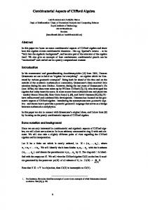
The study of models of self-avoiding loops plays an important role in two-dimensional statistical physics and makes contact with a variety of fields: conformal field theory, integrable systems, algebra and representation theory, combinatorics, and probability theory. A particularly rich and interesting model is obtained by covering all the edges of a (tilted) square lattice with loops which split in one of two possible ways at each bulk vertex, and are reflected at boundary vertices. A possible configuration is shown in Fig. 1. We shall focus on the case where the

Figure 1: Configuration of self-avoiding fully-packed loops on an annulus.

1

overall topology is that of an annulus, with reflecting boundary conditions horizontally, and periodic boundary conditions vertically. The loops can then have two different homotopies with respect to the periodic direction: contractible or non-contractible. In general, we may define a statistical ensemble by giving a weight n to each contractible loop and a weight ℓ to each non-contractible loop. The weight of the configuration in Fig. 1 is then nℓ2 . The model just defined is closely related to the Q-state Potts model, and has the algebraic structure of the Temperley-Lieb algebra. It also has a Uq (sl2 ) quantum group symmetry. In Ref. [1] we have initiated the study of a more general model in which special weights nl and ℓl are given to loops that touch at least once the left boundary. This model has the algebraic structure of the blob algebra (introduced in [2]), which has also been called the one-boundary Temperley-Lieb (1BTL) algebra in recent papers. This latter terminology means that only one of the two boundaries (by convention, the left one) gives rise to special loop weights. In the same spirit, we shall sometimes refer to the ordinary Temperley-Lieb case (with no distinguished boundary) as 0BTL. In our first paper [1], we have mostly elucidated physical features of the one-boundary case, the most mathematical ones having been studied in earlier works [3, 4, 5]. In the limit of an infinitely large lattice, the model turns out to be conformally invariant, and each choice of nl gives rise to a distinct conformal boundary condition. In this second paper, we deal with some combinatorial aspects of the two-boundary case, in preparation for the study of its conformal field theoretic aspects. Our wish to single out the combinatorial treatment is that (most of) the arguments given are completely rigorous, and the results hold true for a lattice of any finite size. Moreover, they are to a large extent independent of the underlying lattice structure, and of the particularities of the model at hand (fully-packing constraint, choice of local vertex weights, etc). They underlying algebraic framework is now the two-blob—or two-boundary Temperley Lieb (2BTL)—algebra [5, 6, 7]. This algebra raises fascinating questions, both of a mathematical nature (representation theory, etc) and of a more physical nature (boundary conformal field theory, etc). In full generality, the weight of a loop in the two-boundary case is then given by the following table: Contractible Yes Yes Yes Yes No No No No

Touches the left boundary No Yes No Yes No Yes No Yes

Touches the right boundary No No Yes Yes No No Yes Yes

Weight n nl nr nb ℓ ℓl ℓr ℓb

(1.1)

It is also appropriate to gather here some other notations that we shall use throughout the paper: N L ei bl , br D d UL
(cos θ) = p q

sin(L+1)θ sin θ

Strip width (number of strands/sites), sometimes written N = 2N2 Number of non-contractible lines Temperley-Lieb (bulk) generator Blob (boundary) generators Dimension of the commutant (eigenvalue amplitude) Dimension of invariant subspace (transfer matrix dimension) Lth order Chebyshev polynomial of the second kind p! Binomial coefficient q!(p−q)! for integer 0 ≤ q ≤ p; zero otherwise

(1.2)

Note that, due to the fully-packing constraint, N and L must have the same parity. In Fig. 1, N = 4 and L = 2. Throughout we shall assume N even, except when the contrary is stated explicitly. This restriction is not essential, and it is imposed mostly in order to write down the simplest formulae only. In sections 2–4 we shall introduce the transfer matrix of the loop model, define the states it acts on, relate it to the underlying algebras, define and compute the dimensions d of its various sectors, and 2

Figure 2: From left to right: identity I and Temperley-Lieb generator ei acting on two strands i and i + 1; left and right boundary identity operator. derive the corresponding eigenvalue amplitudes D (which are also the dimensions of the commutant). To gain clarity, we shall do so gradually, by treating first the ordinary Temperley-Lieb case (0BTL), and then consider next the one- and two-boundary cases. In section 5 we give a more algebraic account on the numbers D, and in section 6 we discuss the determinants of various Gram matrices which occur naturally when studying the representation theory of the boundary Temperley-Lieb algebras. Finally, section 7 is devoted to our conclusions.

2

Zero-boundary case

Although the 0BTL case has long been well understood [8, 9, 10], we shall review it here since it contains many of the elements necessary to attack the cases with boundaries. This approach also has the advantage of fixing a consistent notation and terminology which should facilitate the reading of sections 3–4.

2.1

Algebraic structure

Consider a system of N strands labeled i = 1, 2, . . . , N . The lattice is built up from elementary generators ei , acting on strands i and i + 1, as shown in Fig. 2. More precisely, in the case where all local vertex weights are unity, the transfer matrix reads    N/2 N/2−1 Y Y (I + e2j )  (I + e2j−1 ) (2.1) T = j=1

j=1

The generators ei satisfy the well-known relations e2i

= nei

ei ei±1 ei = ei [ei , ej ] = 0 for |i − j| ≥ 2

(2.2)

The identity and the N − 1 generators ei define the Temperley-Lieb algebra T LN (n), subject to the above relations. Graphically, the application of the last two relations allows to deform and diminish the size of a loop, and when it has reached its minimal possible size it can be taken away and replaced by the weight n due to the first relation.

2.2

States and transfer matrix decomposition

The transfer matrix T acts on states which can be depicted graphically as non-crossing link patterns within a slab bordered by two horizontal rows, each of N points. The complete list of states for N = 4 is shown in Fig. 3. The bottom (resp. top) row of the slab corresponds to time t = 0 (resp. t = t0 ); the transfer matrix propagates the states from t0 to t0 + 1 and thus acts on the top of the slab only. A link joining the top and the bottom of the slab is called a string, and any other link is called an arc. We denote by s the number of strings in a given state. Any state can be turned into a pair of reduced states by cutting all its strings and pulling apart the upper and lower parts. For convenience, a cut string will still be called a string with respect to the reduced state. The complete list of reduced states for N = 4 is shown in Fig. 4.

3

Figure 3: List of all 0BTL states on N = 4 strands. Each row corresponds to a definite sector of the transfer matrix.

Figure 4: List of all 0BTL reduced states on N = 4 strands. Each row corresponds to a definite sector of the transfer matrix.

4

Conversely, a state can be obtained by adjoining two reduced states, gluing together their strings in a unique fashion. Thus, if we define dj as the number of reduced states with s = 2j strings, the number of states with s = 2j strings is simply d2j . The partition function ZN,M on an annulus of width N strands and height M units of time cannot be immediately expressed in terms of reduced states only, since these do not contain the information about how many loops (contractible or non-contractible) are formed when the periodic boundary condition is imposed. We can however write it in terms of states as ZN,M = hu|T M |vi .

(2.3)

At time t0 = 0 the top and the bottom of the slab must be identified. Therefore, the entries of the right vector |vi are one whenever the corresponding state contains no arcs, and each of its links connects a point in the bottom row to the point immediately above it in the top row; all other entries of |vi are zero. At time t0 = M the top and the bottom of the slab must be reglued. Therefore, the left vector hu| is obtained by identifying the top and bottom rows for each state; counting the number of loops of each type gives the corresponding weight as a monomial in the loop weights n and ℓ. The reduced states can be ordered according to a decreasing number of strings. The states can be ordered first according to a decreasing number of strings, and next, for a fixed number of strings, according to its bottom half reduced state. These orderings are brought out by the rows in Figs. 3–4. With this ordering of the states, T has a blockwise lower triagonal structure in the basis of reduced states, since the generator ei can annihilate two strings (if their position on the top of the slab are i and i + 1) but cannot create any strings. In the basis of states, T is blockwise lower triagonal with respect to the number of strings, for the same reason. Each block on the diagonal in this decomposition corresponds to a definite number of strings. The block corresponding to s = 2j strings is denoted T˜j . But since T acts only on the top of the slab, each T˜j = Tj ⊕ . . . ⊕ Tj is in turn a direct sum of dj identical blocks Tj which correspond simply to the action of T on the reduced states with 2j strings. In particular, the eigenvalues of T are the union of the eigenvalues of Tj , where the Tj now act in the much smaller basis of reduced states. This observation is particularly useful in numerical studies.

2.3

The dimensions dL and DL

We briefly review a combinatorial construction [11] which we shall generalize to the case with boundaries in the following sections. We take for now the width of the annulus N = 2N2 to be even. For each transfer matrix block Tj we define the corresponding character as M

Kj = Tr (Tj )

,

(2.4)

where we stress that the trace is over reduced states. Obviously we have Kj =

dj  X

(j)

λi

i=1

M

,

(2.5)

(j)

where λi are the eigenvalues of Tj . The expression of the partition function in terms of transfer matrix eigenvalues is more involved, due essentially to the non-local nature of the loops, and reads ZN,M ≡

N2 X

Zj =

N2 X

D2j Kj ,

(2.6)

j=0

j=0

where Zj is the annulus partition function constrained to have exactly L = 2j non-contractible loops, and D2j are some eigenvalue amplitudes to be determined. To be more precise, we decompose Zj in

5

Figure 5: Construction of invariant reduced states. (a) A configuration contributing to Z2 with N2 = 6, here depicted as a state. (b) Application on the bottom of the reduced state corresponding to the top half of (a). (c) After removal of the arcs one has simply 2j links. terms of Kk as follows Zj

=

N2 X

D(k, j)ℓ2k Kk

(2.7)

k=j

D2j

=

j X

D(j, i)ℓ2i

i=0

and consider next the inverse decomposition Kk =

N2 X

E(j, k)

j=k

Zj . ℓ2j

(2.8)

The determination of the coefficients E(j, k) can be turned into a combinatorial counting problem as follows. First, recall that the characters Kk were defined as traces over reduced states. We must now determine how many times each Zj occurs within a given trace. Consider therefore some configuration C on the annulus that contributes to Zj . An example with j = 2 and N2 = 6 is shown in Fig. 5a. It is convenient not to represent the contractible loops within the configuration, i.e., to depict it as a state. This configuration will contribute to the trace only over such reduced states S that are left invariant by the action of the configuration. Therefore, S must contain the same arcs as does C in its top row (see Fig. 5b). It suffices therefore to determine the parts of S which connect onto the starting points of the 2j non contractible lines (see Fig. 5c). Since the goal is to determine the contribution to Kk , precisely 2k strings and j − k arcs must be used. In other words, E(j, k) is precisely the number of reduced states on 2j strands, and using 2k strings. Now let ∞ X E(j, k)z j (2.9) E (k) (z) = j=0

be the corresponding generating function, where z is a formal parameter representing the weight of an arc, or of a pair of strings. When k = 0, a reduced state with no strings is either empty, or has a leftmost arc which divides the space into two parts (inside the arc and to its right) each of which can accomodate an independent arc state. The generating function f (z) ≡ E (0) (z) therefore satisfies

6

f (z) = 1 + zf (z)2 with regular solution f (z) =

1−

√ ∞ 1 − 4z X (2j)! = zj . 2z j!(j + 1)! j=0

(2.10)

When k 6= 0, the strings simply divide the space into 2k+1 parts each of which contains an independent arc state. Therefore,    ∞  X 2j 2j E (k) (z) = z k f (z)2k+1 = − zj (2.11) j+k j+1+k j=k

and in particular we have dL = E



N L , 2 2



=



   N N − . (N + L)/2 1 + (N + L)/2

(2.12)

Note that dL depends on N , but we usually will not mention this explicitly. Inversion of the linear system (2.8) finally leads to   j+k , D(j, k) = (−1)j+k 2k

(2.13)

which can also be written DL = UL (ℓ/2) , where Uk (x) is the kth order Chebyshev polynomial of the second kind, UL (cos θ) = The total number of states is   N2 X N d2j = . N/2 j=0 One should also note the sum rule

N2 X

d2j D2j = ℓN

(2.14) sin(L+1)θ . sin θ

(2.15)

(2.16)

j=0

which expresses the fact that there are ℓ degrees of freedom living on each site. The representation theory of the 0BTL algebra is of course well-known, as are the links to the XXZ spin chain [5]. For generic values of n, the irreducible representations are labeled by a single integer L = 0, 2, . . . , N which counts the number of non-contractible (or “through”) lines, and have dimension equal to the multiplicity of the spin L2 representation in a chain of N spins 1/2. This dimension is easily seen to be dL of (2.12). Meanwhile, DL is a q-dimension for the corresponding commutant (the quantum algebra Uq (sl2 ) with q + q −1 = l.

2.4

The odd and dilute cases

Although we have showed how to obtain dL and DL only for a somewhat particular case (with N even, and for a fully-packed model of loops) the results hold true more generally. That the expressions (2.12) for dL and (2.14) for DL are correct also for N (and hence L) odd is actually obvious from the way they are derived. As an additional check, note that the sumrule for the odd case indeed becomes ⌊N/2⌋ X d2j+1 D2j+1 = ℓN . (2.17) j=0

For the dilute case, where not all of the N sites need sustain a link, the number of states dL obviously changes. To see how, let now z˜ be the weight of one site (recall that z was previously defined as the weight of two sites). Let f˜(˜ z ) be the generating function of a state consisting only of arcs and empty sites. If such a state is non-empty, it contains a first site which can either be empty or occupied 7

Figure 6: Operators acting on the left boundary. From left to right: identity, blob, fork. by an arc. In the former case, the remainder of the state is again an arc state, and in the latter the leftmost arc divides space into two parts which can each sustain an independent arc state. We have z )2 with regular solution therefore f˜(˜ z ) = 1 + z˜f˜(˜ z ) + z˜2 f˜(˜ ! √ j+2 ∞ j+2−k −(j+2) 2 X X 1 − 2˜ z − 3˜ z 1 − z ˜ − 3 2 (2k − 2)! z˜j (2.18) f˜(˜ z) = = 2˜ z2 (k − 1)! (j + 2 − k)! (2k − j − 2)! j=0 k=1

The number inside the parenthesis is known in combinatorics as the jth Motzkin number [12]. The generating function for dilute states with L strings is then z )L+1 = z˜L f˜(˜

∞ X

ddil zj L (N = j)˜

(2.19)

j=L

and defines the dilute dimensions ddil L (N ). We now claim that the dimensions DL of (2.14) are unchanged in the dilute case. While this can be seen be repeating the construction of invariant reduced states, we shall opt instead for a simple check. Indeed, the sumrule with ddil L as above and DL taken from (2.14) becomes N X

N ddil L DL = (ℓ + 1)

(2.20)

L=0

where we note that the sum is now over both parities of L. This result is exactly as expected, since the number of degrees of freedom living at each site must indeed be ℓ + 1 (with ℓ coming from the loops, and 1 coming from the possibility of the site being empty). In the 1BTL and 2BTL cases treated below, similar extensions to the odd and dilute cases may be worked out. However, since we have just seen on the simpler 0BTL example that the dimensions DL —our main concern—are unchanged, we shall not go through this exercise in what follows.

3 3.1

One-boundary case Algebraic structure

In the one-boundary case, contractible loops touching at least once the left boundary receive a weight nl which is different from the weight n of a bulk loop. Coding this algebraically requires the introduction of an additional generator bl acting on the (left) boundary, such that b2l

=

e1 bl e1 = [bl , ei ] =

bl nl e 1 0 for i = 2, 3, . . . , N − 1

(3.1)

These relations, with (2.2), define the one-boundary Temperley-Lieb (1BTL) algebra [2]. Graphically, the action of bl can be depicted by adding a blob (shown in the following figures as a circle) to the link that touches the boundary. This is illustrated in Fig. 6. The first relation in (3.1) means that all the anchoring points of a boundary touching loop, except the last one, can be taken away. The third relation and (2.2) allow to deform and diminish the size of a boundary loop (while keeping it glued to one of its anchoring points on the boundary), and when it has reached its minimal possible size it can be taken away and replaced by the weight nl due to the second relation of (3.1). 8

Figure 7: List of all 1BTL states on N = 4 strands (with λl = 0). Each row corresponds to a definite sector of the transfer matrix. In part of the literature (see [13] for an example) the algebra (3.1) is normalized differently, and the boundary generator is depicted as a fork rather than a blob (see Fig. 6). This means that where a loop touches the boundary it is cut, and the two ends are attached to the boundary. This convention allows to interpret a loop touching the boundary k times as a collection of k half loops with end points on the boundary. These half loops can subsequently be pulled apart, something which is not possible in the blob picture. In this paper we shall work exclusively in the blob picture, but we believe that all our results can equivalently be derived and interpreted in the fork picture. The transfer matrix can be taken as    N/2 N/2−1 Y Y (I + e2j )  (I + e2j−1 ) (λl I + bl ) (3.2) T = j=1

j=1

where a non-zero value of λl would mean that with some probability a loop may come close to the boundary without actually touching it. We will mostly set λl = 0 in what follows. This has the advantage of reducing the dimension of the space on which T acts, since then the leftmost link in any (reduced) state may be taken to be blobbed. The algebraic results for the case λl 6= 0 are simply related to those for the case λl = 0, and we shall discuss them in due course.

3.2

States and transfer matrix decomposition

The states of the transfer matrix are as in the 0BTL case, except that links which are exposed to the boundary (i.e., which are not to the right of the leftmost string) may be blobbed. Also, any link touching the leftmost site (i = 1) is necessarily blobbed, since we have taken λl = 0 in (3.2). The states for N = 4 are shown in Fig. 7, and the corresponding reduced states are given in Fig. 8. When a blobbed and an unblobbed link are adjoined (e.g., when transfering, or when forming an inner product) the result is a blobbed (restricted) link.

9

Figure 8: List of all 1BTL reduced states on N = 4 strands (with λl = 0). Each row corresponds to a definite sector of the transfer matrix. It should be noted that there is a slightly different way [2] of defining the 1BTL states by projecting the unblobbed links onto the orthogonal complement of the blobbed ones, i.e., associating them with 1 − bl . These links can be decorated with another symbol (taken to be a small square in Ref. [2]). A squared loop now comes with a weight n − nl , and when a blobbed and a squared link are adjoined the result is zero by orthogonality. Clearly, the two constructions are completely equivalent. We shall not use the alternate definition in this paper. The decomposition of the transfer matrix into sectors (blocks) takes place exactly as in the 0BTL case, with one important addition. Namely, once the number of strings s = 2j has been fixed, the blocks Tj are blockwise 2 × 2 lower triangular with respect to the blobbing status of the leftmost string. Indeed, acting by bl can blob the leftmost string, but a string—qua a conserved object with respect to Tj —cannot subsequently be unblobbed. The elementary blocks are therefore Tjb and Tju , where the superscript indicates the blobbing status (b for blobbed, and u for unblobbed) of the leftmost string. With λl = 0, there is no unblobbed sector with j = N/2, and by convention the sector with j = 0 is unblobbed (for any λl ). In Figs. 7–8, the second rows give the unique unblobbed state with j = 1.

3.3

The dimensions dαL

Let us now determine the number of reduced states in the various sectors of the transfer matrix. Recall that (2.10) gives the generating function f (z) of a collection of unblobbed arcs. We shall also need the generating function e(z) of arc states, where exterior arcs are allowed (but not required) to be blobbed, and all interior arcs are unblobbed. Such a state is either empty, or it has a leftmost arc (which may or may not be blobbed) which divides the space into two parts (inside the arc and to its right). On the inside is a collection of unblobbed arcs (i.e., a factor of f (z)), and on the right is another factor of e(z). Thus, e(z) = 1 + 2zf (z)e(z), or ∞   X 2j j 1 z . (3.3) = e(z) = √ j 1 − 4z j=0 Consider now first the case of λl 6= 0 in (3.2), where the leftmost object may have any blobbing status. If the left string is required to be unblobbed, the generating function in the sector with 2k strings is  ∞  X 2j k 2k e(z)z f (z) = zj , (3.4) j−k j=k

and the result is the same if the left string is required to be blobbed. Thus,   N duL = dbL = (For λl 6= 0) (N − L)/2

(3.5)

This is a well-known result for the 1BTL algebra [2]. Note in particular that the total number of states is N2 N2 X X db2j = 2N . (3.6) du2j + j=0

j=1

10

Consider next the case of λl = 0, the convention that we shall use below, and for which Figs. 7–8 apply. In the blobbed sector we must distinguish the case where the leftmost object is a string or an arc. This gives  ∞  X 2j − 1 j z k f (z)2k + z k+1 e(z)f (z)2k+1 = z . (3.7) j−k j=k

Meanwhile, for the unblobbed sector, the leftmost object must be a blobbed arc. The generating function then reads  ∞  X 2j − 1 z k+1 e(z)f (z)2k+1 = zj . (3.8) j−k−1 j=k

To summarize, we have shown that there are two different types of irreducible representations (unblobbed and blobbed), obtained by acting with the algebra on reduced states, of dimensions     N −1 N −1 u b dL = , dL = (For λl = 0) (3.9) (N − L)/2 − 1 (N − L)/2 The total number of states is now NX 2 −1 j=0

du2j +

N2 X

db2j = 2N −1 .

(3.10)

j=1

Note that in the papers [4, 5], the whole algebra is considered, corresponding to our case λl 6= 0. We shall however continue to study the simpler quotient (λl = 0) below.

3.4

The dimensions DLα

In what follows, Greek letters α and γ are sector labels which can designate the blobbed (α = b) or the unblobbed (α = u) sector. The character Kjα corresponding to a transfer matrix block Tjα is defined as
M , (3.11) Kjα = Tr Tjα

the trace being over reduced states. The constrained annulus partition function Zjα is defined to have exactly 2j non-contractible loops, of which the leftmost is blobbed or unblobbed according to the value of α. Recall that the number of strands N = 2N2 is assumed to be even. The allowed values of j in (3.11) are then For Kju : j = 0, 1, . . . , N2 − 1 (3.12) For Kjb : j = 1, 2, . . . , N2 and similarly for the Zjα . The decomposition of the constrained partition functions reads Zjα =

N2 X   α Du (k, j)ℓ2k Kku + Dbα (k, j)ℓl ℓ2k−1 Kkb ,

(3.13)

k=j

where Dγα (k, j) are coefficients to be determined. They define the amplitudes of the transfer matrix eigenvalues j X  α  α Du (j, i)ℓ2i + Dbα (j, i)ℓl ℓ2i−1 . (3.14) D2j = i=0

As in the 0BTL case, we turn the problem upside down and consider the inverse decomposition # " N2 X Zjb Zju α α α (3.15) Kk = Eu (j, k) 2j + Eb (j, k) 2j−1 . ℓ ℓl ℓ j=k

11

The coefficient Eγα (j, k) counts how many times each Zjγ occurs in a given trace Kkα . Just as in the 0BTL case this means that we must count the number of invariant reduced states on 2j strands, using 2k strings and j − k arcs. The construction is the same as shown in Fig. 5, with an important modification: γ now gives the blobbing status of the leftmost string in Fig. 5c, and α gives the blobbing status of the leftmost string in the sought-for invariant reduced state. The number of different families of coefficients Eγα (j, k) to be determined is actually three rather than four. More precisely we have E1 E2 E3

≡ Euu = Eub

≡ Ebu ≡ Ebb

(3.16)

defining Eσ (j, k) for σ = 1, 2, 3. The corresponding generating functions Eσ(k) (z) =

∞ X

Eσ (j, k)z j

(3.17)

j=0

can then be written down in terms of those of states of unblobbed arcs f (z) [see (2.10)], and of arc states where any exterior arc may be blobbed e(z) [see (3.3)]. This gives:  ∞  X 2j (k) E1 (z) = z k e(z)f (z)2k = zj j−k j=k  ∞  X 2j − 1 (k) k+1 2k+1 E2 (z) = z e(z)f (z) = zj (3.18) j−k−1 j=k+1  ∞  X 2j − 1 j (k) E3 (z) = z k f (z)2k (1 + ze(z)f (z)) = z j−k j=k

The linear system (3.15) with (3.18) can now be inverted, leading to the result u DL

= UL (ℓ/2) − ℓl UL−1 (ℓ/2)

b DL

= ℓl UL−1 (ℓ/2) − UL−2 (ℓ/2)

(3.19)

when expressed in terms of Un (x), the nth order Chebyshev polynomial of the second kind. [Note carefully that we have here defined Un (x) = 0 on the right-hand side when n < 0, which is a nonstandard choice.] Using the identity Un (x) = 2xUn−1 (x) − Un−2 (x) (3.20) we get the following reductions from the 1BTL case to the 0BTL case: u DL |ℓ =ℓ l b D L ℓl =ℓ

= −UL−2 (ℓ/2) ≡ −DL−2 = UL (ℓ/2) ≡ DL

(3.21)

For the sumrule giving the size of the total Hilbert space there are two choices for the dα j . When λl 6= 0 in (3.2) one has (3.5), giving N2 X

u du2j D2j +

j=0

N2 X

b db2j D2j = ℓN .

(3.22)

j=1

When λl = 0 one has (3.9), giving instead NX 2 −1 j=0

u du2j D2j +

N2 X

b db2j D2j = ℓl ℓN −1 .

j=1

12

(3.23)

This latter result expresses clearly that the number of degrees of freedom on the first strand has been reduced from ℓ to ℓl . These two sumrules are also an important check of the fact that the dimensions α DL depend only on the number of non-contractible lines, and not on how one restricts the states of the transfer matrix.

4 4.1

Two-boundary case Algebraic structure

In the two-boundary case, a contractible loop has four different possibilities: it can touch none of the boundaries, only the left one, only the right one, or touch both boundaries. The corresponding weights have already been defined in (1.1). Algebraically we still have the relations (2.2) and (3.1). We shall also need the analogue of (3.1) on the right boundary: b2r

= br

eN −1 br eN −1 = nr eN −1 [br , ei ] = 0 for i = 1, 2, . . . , N − 2

(4.1)

Obviously, the time order in which a loop touches the two boundaries does not affect its weight, so we should further set [bl , br ] = 0 . (4.2) For fixed N , the above relations now give an infinite number of words, since we have not yet given a prescription for how to “dispose of” loops touching both boundaries. We shall therefore need to take the following quotient         N/2 N/2 N/2−1 N/2 Y Y Y Y  e2j−1  . (4.3) e2j−1  = nb  e2j  bl  e2j−1  br  j=1

j=1

j=1

j=1

Graphically, this expresses that the smallest possible loop extending from left to right, and blobbed on both sides, can be taken out and replaced by a factor of nb . The remaining relations then suffice to ensure this weighting for a loop of any size and shape touching the two boundaries. We emphasize again that our diagrammatic conventions are in terms of the blob picture, rather than the fork picture [13] which has been discussed briefly in section 3.1. In the fork picture it is natural to exploit the fact that half loops can be pulled apart to replace the single quotient (4.3) by a double quotient [7]. This is however meaningless in the blob picture. Note also that the sector labels (“blobbed” and “unblobbed”) in the blob picture (to be discussed below) are analogous to the parity of connections to the left and right boundaries in the fork picture (see Definition 4.2 of Ref. [7]). Needless to say, the two approaches had better agree on the dimensions of the irreducible representations of 2BTL (and we shall see below that indeed they do). The transfer matrix can be taken as     N/2 N/2−1 Y Y (I + e2j ) (λr I + br )  (I + e2j−1 ) (λl I + bl ) (4.4) T = j=1

j=1

where non-zero values of λl and λr mean (as in the 1BTL case) that with some probability a loop may come close to a boundary without actually touching it. We have already seen in the 1BTL case how the choice of these parameters changes slightly the counting of states, and the sumrules linking dL and DL . We now wish to determine with which amplitudes the eigenvalues of the transfer matrix T enter into the annulus partition function. These amplitudes, which can also be interpreted as operator multiplicities, depend only on the weights of non contractible loops (ℓ, ℓl , ℓr , and ℓb ). In particular, 13

Figure 9: List of all 2BTL reduced states on N = 4 strands (with λl = λr = 0). Each row corresponds to a definite sector of the transfer matrix. they are independent of the lattice structure, local occupancy constraints (fully-packed or dilute case), and of local vertex weights. The amplitudes are also independent of the weights of contractible loops, as long as these are non-zero (but they do depend on whether nb = 0 or nb 6= 0, as discussed in details below). To simplify the discussion we shall henceforth deal with the fully-packed model only.

4.2

States and transfer matrix decomposition

Let T be the 2BTL transfer matrix (4.4). The concept of states, made up of links which are arcs or strings, has already been defined in the 0BTL case. The states on which T acts are as in the 1BTL case, except that links which are exposed to the right boundary (i.e., which are not to the left of the rightmost string) may be blobbed by the second boundary generator br . It is necessary to introduce distinct symbols for the left blob (a circle) and the right blob (a square). The reduced states for N = 4 are shown in Fig. 9. Let s be the number of strings in a given state. Note that T cannot change the parity of s. We have therefore T = Teven ⊕ Todd . As usual we assume N = 2N2 even, and so the partition function

 even M ZN,M = u|Teven |v . (4.5)

is constrained to an even number of non contractible lines. Note that the loop weight ℓb cannot appear in Z even (and similarly nb cannot appear in Z odd ). Henceforth we shall drop the epithet “even”. Only the leftmost string, and the arcs to its left, can be blobbed by bl . Similarly, only the rightmost string, and the arcs to its right, can be blobbed by br . When s = 0, at most one arc can be blobbed on both sides (i.e., by bl br ). If there is such a doubly blobbed arc, any arc to its left (resp. right) cannot be blobbed by br (resp. bl ). When nb = 0 doubly blobbed arcs are forbidden, so in the sequel we shall have to distinguish between the cases nb = 0 and nb 6= 0. (To compute Zodd we would similarly have to distinguish between ℓb = 0 and ℓb 6= 0, when s = 1). The states can be ordered as follows: First we sort the states according to a decreasing number of strings s. For fixed s > 0, we place first the states in which the leftmost and rightmost strings are both unblobbed (henceforth called uu states), then states in which only the rightmost string is blobbed (ub states), then states in which only the leftmost string is blobbed (bu states), and finally states in which both the leftmost and rightmost strings are blobbed (bb states). Having done this, we finally group together states (with fixed s and fixed blobbing (uu, ub, bu, or bb) of the outermost strings) that possess an equal lower-half reduced state. With this ordering of the states, T has a lower block-triagonal structure, with each block corresponding to a group of states as defined above. The blocks on the diagonal of T are denoted Tjαβ , where j = s/2 is the number of pairs of strings, and the indices α, β = u or b. Note that the blocks Tjαβ can be constructed in terms of the reduced states.

14

4.3

The dimensions DLαβ

In what follows α, β, γ, δ = u or b are sector labels. For each transfer matrix block Tjαβ we define the corresponding character as M  Kjαβ = Tr Tjαβ , (4.6)

where as usual the trace is over reduced states. Also, let Zjαβ be the annulus partition function constrained to have exactly j non contractible loops, of which the leftmost (resp. rightmost) has blobbing status α (resp. β). For example, Zjub consists of the terms in the full partition function ZN,M whose dependence on ℓ, ℓl , ℓr is precisely ℓ2j−1 ℓr . The allowed values of j in (4.6) are then For Kjuu For Kjub and Kjbu For Kjbb

: : :

j = 0, 1, . . . , N2 − 2 j = 1, 2, . . . , N2 − 1 j = 1, 2, . . . , N2

(4.7)

and similarly for the Zjαβ . All other characters and constrained partition functions are defined to be zero in order to lighten the notation in the following formulae. The goal is now to search for a decomposition of the form Zjαβ

=

N2 h X

αβ αβ Duu (k, j)ℓ2k Kkuu + Dub (k, j)ℓ2k−1 ℓr Kkub

k=j

+

αβ αβ Dbu (k, j)ℓl ℓ2k−1 Kkbu + Dbb (k, j)ℓl ℓ2k−2 ℓr Kkbb

i

(4.8)

αβ where Dγδ are coefficients to be determined. The complete amplitude—here constructed combinatorially monomial by monomial—then reads

αβ D2j

j h i X αβ αβ αβ αβ Duu (j, i)ℓ2i + Dub (j, i)ℓ2i−1 ℓr + Dbu (j, i)ℓl ℓ2i−1 + Dbb (j, i)ℓl ℓ2i−2 ℓr . =

(4.9)

i=0

The inverse decomposition of Kk in terms of Zj reads # " N2 ub bu bb uu X Z Z Z Z j j j j αβ αβ αβ αβ αβ Euu (j, k) 2j + Eub (j, k) 2j−1 + Ebu (j, k) 2j−1 + Ebb (j, k) 2j−2 Kk = ℓ ℓ ℓr ℓl ℓ ℓl ℓ ℓr

(4.10)

j=k

αβ The coefficients Eγδ (j, k) counts how many times each Zjγδ occurs in a given trace Kkαβ , expressed in terms of invariant reduced states on 2j strands, using 2k strings. αβ The various symmetries in the problem reduce the number of families of coefficients Eγδ (j, k) to be determined from sixteen to six. More precisely we have:

E1 E2 E3 E4 E5 E6

uu ub bu bb ≡ Euu = Euu = Euu = Euu

bu ub uu uu ≡ Eub = Ebu = Eub = Ebu uu ≡ Ebb

(4.11)

ub bu bb bb ≡ Eub = Ebu = Eub = Ebu ub bu ≡ Ebb = Ebb

bb ≡ Ebb

defining Eσ (j, k) for σ = 1, 2, . . . , 6. To count the corresponding number of invariant states we introduce the diagrammatic symbols shown in Fig. 10. Now let ∞ X Eσ (j, k)z j (4.12) Eσ(k) (z) = j=0

15

(a)

(b)

(c)

(d)

11111111 00000000 00000000 11111111 00000000 11111111 00000000 11111111 00000000 11111111

111111111 000000000 000000000 111111111 000000000 111111111 000000000 111111111 000000000 111111111

(e)

(f)

Figure 10: Diagrams representing (a) an unblobbed arc, (b) a blobbed arc, (c) an unblobbed string, (d) a blobbed string, (e) a collection of arcs of which exterior arcs may (but need not) be blobbed, and (f) a collection of arcs of which all exterior arcs are unblobbed.

E1

111111111 000000000 000000000 111111111 000000000 111111111 000000000 111111111

111111111 000000000 000000000 111111111 000000000 111111111 000000000 111111111

11111111 00000000 00000000 11111111 00000000 11111111 00000000 11111111

11111111 00000000 00000000 11111111 00000000 11111111 00000000 11111111

E2

11111111 00000000 00000000 11111111 00000000 11111111 00000000 11111111 00000000 11111111

111111111 000000000 000000000 111111111 000000000 111111111 000000000 111111111 000000000 111111111

11111111 00000000 00000000 11111111 00000000 11111111 00000000 11111111 00000000 11111111

11111111 00000000 00000000 11111111 00000000 11111111 00000000 11111111 00000000 11111111

11111111 00000000 00000000 11111111 00000000 11111111 00000000 11111111 00000000 11111111

E3

11111111 00000000 00000000 11111111 00000000 11111111 00000000 11111111 00000000 11111111

111111111 000000000 000000000 111111111 000000000 111111111 000000000 111111111 000000000 111111111

11111111 00000000 00000000 11111111 00000000 11111111 00000000 11111111 00000000 11111111

11111111 00000000 00000000 11111111 00000000 11111111 00000000 11111111 00000000 11111111

11111111 00000000 00000000 11111111 00000000 11111111 00000000 11111111 00000000 11111111

E4

00000000 11111111 11111111 00000000 00000000 11111111 00000000 11111111 00000000 11111111

000000000 111111111 111111111 000000000 000000000 111111111 000000000 111111111 000000000 111111111

00000000 11111111 11111111 00000000 00000000 11111111 00000000 11111111 00000000 11111111

00000000 11111111 11111111 00000000 00000000 11111111 00000000 11111111 00000000 11111111

00000000 11111111 11111111 00000000 00000000 11111111 00000000 11111111 00000000 11111111

111111111 000000000 000000000 111111111 000000000 111111111 000000000 111111111 000000000 111111111

00000000 11111111 11111111 00000000 00000000 11111111 00000000 11111111 00000000 11111111

000000000 111111111 111111111 000000000 000000000 111111111 000000000 111111111 000000000 111111111

000000000 111111111 111111111 000000000 000000000 111111111 000000000 111111111 000000000 111111111

Figure 11: Diagrammatics corresponding to the generating functions Eσ (z) with σ = 1, 2, 3, 4. be the corresponding generating function, where z is a formal parameter representing the weight of an arc, or of a pair of strings. We shall also need the generating functions e(z) and f (z) corresponding to the diagrams (e) and (f) in Fig. 10. In Eqs. (3.3) and (2.10) these have already been found to be ∞   X 2j j 1 z , e(z) = √ = j 1 − 4z j=0

f (z) =

1−

√ ∞ 1 − 4z X (2j)! = zj . 2z j!(j + 1)! j=0

(4.13)

(k)

In terms of these the generating functions Eσ (z) can be written down by respecting carefully the invariance of the states. This is shown diagramatically for for a few sample cases (σ = 1, 2, 3, 4) in Fig. 11. In algebraic terms we have then (k)

z k e(z)2 f (z)2k−1

(k)

z k+1 e(z)2 f (z)2k

E3 (z) =

(k)

z k+2 e(z)2 f (z)2k+1

(k) E4 (z) (k) E5 (z) (k) E6 (z)

=

z k e(z)f (z)2k−1

=

z k+1 e(z)f (z)2k

=

z k f (z)2k−1 1 + 2ze(z)f (z) + z 2 e(z)2 f (z)2

E1 (z) = E2 (z) =


1 + ze(z)f (z)
1 + ze(z)f (z)

(4.14)




It should be stressed that these expressions have been worked out diagramatically by supposing the number of strings 2k > 0. But the first three functions actually enter also into expressions with k = 0. It can be checked that the generating functions (4.14) are still correct upon setting k = 0, provided 16

that we accept that no arc is allowed to be blobbed simultaneously on the left and on the right, i.e., provided that we set nb = 0 in the notation of (1.1). Let us therefore suppose that nb = 0 for now, and return to the issue of nb 6= 0 later on. The linear system (4.10) with (4.14) can now be inverted and brought into the form (4.8). The results for the amplitudes (4.9) have a rather simple form uu DL

=

ub DL bu DL

= =

bb DL

=

UL (ℓ/2) − (ℓl + ℓr )UL−1 (ℓ/2) + ℓl ℓr UL−2 (ℓ/2)

ℓr UL−1 (ℓ/2) − (1 + ℓl ℓr )UL−2 (ℓ/2) + ℓl UL−3 (ℓ/2) ℓl UL−1 (ℓ/2) − (1 + ℓl ℓr )UL−2 (ℓ/2) + ℓr UL−3 (ℓ/2)

(4.15)

ℓl ℓr UL−2 (ℓ/2) − (ℓl + ℓr )UL−3 (ℓ/2) + UL−4 (ℓ/2)

when expressed in terms of Un (x), the nth order Chebyshev polynomial of the second kind. [Note again that we have defined Un (x) = 0 on the right-hand side when n < 0, which is a non-standard choice.] This is the main result of this section. Using the identity (3.20) it is easy to show that we have reduction from the two-boundary to the one-boundary case provided that the boundary which is non-distinguished in the latter case were blobbed in the former. More precisely we find that bb b ub u DL , DL = DL . (4.16) = DL ℓr →ℓ ℓr →ℓ A slightly more curious set of identities results when we remove the distinction of an unblobbed boundary. We have then bu b uu u DL = −DL−2 , DL |ℓr →ℓ = −DL−2 . (4.17) ℓr →ℓ

Finally, (3.20) permits to prove the fusion identity b bb bb b D2b ℓ →ℓr · DL = DL+2 + DL + DL−2 l

(4.18)

where we stress that the last term on the right-hand side is a one-boundary amplitude. More complicated fusion identities can be proved in the same manner. The algebraic origin of these identities will be discussed in the following section.

4.4

The dimensions dαβ L

We must now compute the transfer matrix dimensions dαβ L in the various sectors αβ. Recall that these are expected to depend on the choice of λl and λr in the transfer matrix (4.4). Define the index γ = u (resp. γ = b) if λl 6= 0 (resp. λl = 0). Similarly define the index δ = u or b in terms of λr . A renewed inspection of the diagrammatics of Fig. 11 then reveals that we have simply αβ dαβ L (γδ) = Eγδ (N/2, L/2) ,

(4.19)

αβ where the coefficients Eγδ (j, k) are those of the preceding subsection; see Eq. (4.12). Consider in particular the case of the full 2BTL algebra (with λl 6= 0 and λr 6= 0) for which (4.12) αβ N/2 gives dαβ in the development of L = Euu = E1 independently of α and β. The coefficient of z L/2 E1 (z), given explicitly in (4.14), then yields exactly the dimension of an irreducible representation of the 2BTL algebra, in complete agreement with Proposition 4.1 of Ref. [7]. As already announced in section 4.1, this furnishes a highly non-trivial check that the blob and fork pictures lead to equivalent results. Our interpretation of the irreducible modules (transfer matrix blocks) is however quite different from that of the fork picture [7]. To make this point clear, we invite the reader to compare Figure 5 of Ref. [7] with our Fig. 12. Both show the organization of the irreducible modules and their dimensions for a system on N = 4 strands. In Fig. 13 we give the similar picture for the restricted 2BTL algebra (λl = λr = 0).

17

1

1

1

1

5

5

5

5

16 Figure 12: Organization of transfer matrix blocks (irreducible modules) on N = 4 strands for the full 2BTL algebra (λl 6= 0, λr 6= 0 and nb 6= 0). For each block we show its dimension and one representative state. Undecorated arrows denote transitions induced by the TL generators ei . Arrows decorated by a circle (resp. a square) denote transitions induced by the left (resp. right) boundary generator bl (resp. br ).

1

1

3

1

4 Figure 13: Same as Fig. 12, but for the restricted 2BTL algebra (λl = λr = 0 and nb 6= 0).

18

The following sumrules on the dimensions are readily established: γδ = uu

:

N2 X

uu duu 2j D2j +

γδ = ub

:

uu duu 2j D2j +

γδ = bu

:

uu duu 2j D2j +

γδ = bb

:

uu duu 2j D2j +

j=0

bu dbu 2j D2j +

ub dub 2j D2j +

NX 2 −1

NX 2 −1

N2 X

NX 2 −1

bu dbu 2j D2j +

N2 X

bu dbu 2j D2j +

j=1

bb N −1 dbb ℓr 2j D2j = ℓ

NX 2 −1

N2 X

bb N −1 dbb 2j D2j = ℓl ℓ

j=1

j=1

ub dub 2j D2j +

N2 X j=1

j=1

ub dub 2j D2j +

bb N dbb 2j D2j = ℓ

j=0

j=0

N2 X

j=1

j=0

NX 2 −2

N2 X

j=1

j=0

NX 2 −1

ub dub 2j D2j +

j=0

j=0

NX 2 −1

N2 X

bu dbu 2j D2j +

j=1

N2 X

bb N −2 dbb ℓr 2j D2j = ℓl ℓ

(4.20)

j=1

where we draw the reader’s attention to the summation limits. The total number of states, for instance when λl = λr = 0, is NX 2 −2

duu 2j +

j=0

NX 2 −1

dub 2j +

j=1

NX 2 −1

dbu 2j +

N2 X

dbb 2j =

j=1

j=1

NX 2 −1 k=0

   2k + 1 2N2 − 2 2(k + 1) N2 + k N2 − k − 1 2

(4.21)

The numerical values of this for N = 2, 4, 6, . . . are the following: 1, 7, 35, 162, 723, 3158, . . ..

4.5

Allowing doubly blobbed arcs

Removing the restriction nb = 0 changes our results, since now a single arc is allowed to touch both boundaries. This quests us to recompute E1 (z), E2 (z) and E3 (z) for the case of k = 0 strings. Skipping the details, the results are simply: (0)

E1 (z) =

1 , 1 − 4z

(0)

E2 (z) =

2z , 1 − 4z

(0)

E3 (z) =

z 1 − 4z

for k = 0 and nb 6= 0 .

(4.22)

Inverting again (4.10) leads to exactly the same result (4.15) as before, with one exception: the former result D2bb = ℓl ℓr gets replaced by D2bb = ℓl ℓr − 1

for nb 6= 0 .

(4.23)

αβ Despite of this modification of the DL , the sumrules (4.20) still hold true.

5

The algebraic significance of the D numbers

The d numbers are clearly dimensions of (generically) irreducible representations of the various versions of the Temperley Lieb algebra. As discussed briefly in our first paper [1], the D numbers also have an interesting algebraic interpretation which we would like to elaborate now. The general idea is to interpret the loop configurations in the model (either in the dense or dilute case) as the graphical expansion of an O(n) type model of vector spins, each spin located at a lattice vertex. This generalizes the well-known construction of the bulk O(n) model to a model with boundary. Bulk spins take values in a space of dimension n, hence bulk loops get a fugacity n. The rules for the one-boundary loop model for instance correspond now to constraining boundary spins to take values in a smaller space of dimension nl . Blobbed links then indicate that the spins have been restricted to the smaller space, while unblobbed links indicate no restriction. When a blobbed and an unblobbed link are adjoined (e.g., when transfering, or when forming an inner product) the result is a blobbed (restricted) link. In a model with genuine O(n) symmetry, the D numbers should be the dimensions of irreducible representations of the symmetry group, since they would then be multiplicities of eigenvalues. For 19

instance, the multiplicity n should come with the eigenvalue associated with the order parameter, etc. The slightly more formal structure behind this is a decomposition of the Hilbert space of such an O(n) model into a sum of products of representations of the symmetry times representations of the commutant. The question then is to adapt these ideas to the case of loop models. While loop models for arbitrary values of the parameter n are difficult to fully understand in terms of symmetry, such an understanding was recently achieved [14] for integer (positive or negative) values of n. We propose here to interpret the 1BTL and 2BTL algebra and the D numbers within this framework. We start with some reminders. A cursory look at the D numbers in the ordinary TL case reveals quantities which, for n integer, do not reproduce dimensions of irreducibles of O(n), but allow for considerably higher degeneracies! The point is that the dense model has a much larger symmetry than O(n). Since loop crossings are not allowed, one can expect at least the symmetry U(n); a closer look shows that this symmetry is in a certain sense realized “locally”, giving rise to a yet larger symmetry algebra dubbed An in [14]. A convenient way to understand the enlarged symmetry is to give explicit expressions for all its generators. This was done in [14] and we start by recalling some results from this reference. We first consider the case n a positive integer, and a Hilbert space made of N = 2N2 sites labelled i = 1, . . . , N , with an n-dimensional complex vector space Vi = Cn at each site. The states can be a† represented using oscillator operators bai , b†ia for i even, bia , bi for i odd, with commutation relations [bai , b†jb ] = δij δba (where a, b = 1, 2, . . . , n), and similarly for i odd. The destruction operators bai , bia destroy the vacuum state, the daggers indicate the adjoint, and the spaces Vi are defined by the constraints b†ia bai

=

1

(i even),

(5.1)

a† bi bia

=

1

(i odd)

(5.2)

of one boson per site (we use the summation convention for repeated indices of the same type as b a). We define the generators of SU(n) (or in fact of gln ) acting in the spaces Vi by Jia = b†ia bbi for b†

b i even, Jia = −bi bia for i odd, and the commutation relations among the P Jibs (for each i) are i, acts in the tensor independent. Hence the global gln algebra, defined by its generators Jab = i Jia product V = ⊗N V of copies of the fundamental representation of gl on even sites, alternating with i m i=1 its dual on odd sites. Though the U(1) subalgebra of gln generated by Jaa acts trivially on the chain (and by a scalar on each site), it is often notationally convenient not to subtract this trace from the generators Jab . The invariant nearest-neighbor coupling in the chain is unique, up to additive and multiplicative constants. It is the usual “Heisenberg coupling” of magnetism, and can be written in terms of operators ei , defined explicitly as ( a† bi+1 b†ia bbi bi+1,b , i even, ei = (5.3) a† bi b†i+1,a bbi+1 bib , i odd.

The ei ’s are Hermitian, e†i = ei . Acting in the constrained space V , they satisfy the usual TL relations (2.2).

5.1

Zero-boundary case

In the case of ordinary (0BTL) boundary conditions, the numbers DL are the dimensions DL of the Lth representation of the commutant of TLN (n) in V . These numbers can be found inductively, by adding another pair of non-contractible dots to the end of a sequence. This leads easily to the recurrence relation1 D2 DL = DL+2 + DL + DL−2 . (5.4) which is illustrated pictorially in Fig. 14. 1 In

some of our other papers, labels for the representations are SU (2) spins, and thus one half of those used here.

20

Figure 14: Fusion in the ordinary TL model. Also, it is clear that the initial values read D0 = 1 and D2 = n2 − 1 [note that D2 is the dimension of the adjoint representation of SU(n)]. The solution is DL = UL (n/2). For n > 2, these dimensions increase exponentially with L. Note that these dimensions are the multiplicities of energy eigenvalues for any of the transfer matrices/hamiltonians built using the Temperley Lieb algebra (barring accidental degeneracies). We thus recover the result (2.14) in the case ℓ = n. The whole construction (this will be emphasized more below) is in fact identical when contractible and non contractible lines carry a different weight, and formally depends only on the latter; the result can thus be used in the case ℓ 6= n as well, reproducing now (2.14) in all cases. The commutant algebra can be constructed explicitly as follows. We introduce the operators (for k ≤ N) X ...ak Jeba11ba22...b = Jia11b1 Jia22b2 · · · Jiakkbk (5.5) k 1≤i1 1: b b b b DL (n2 − 1) = DL+2 + DL + DL−2 u u u u DL (n2 − 1) = DL+2 + DL + DL−2

(5.8)

and the solution is easily seen to coincide with (3.19) in the case ℓ = n. The relations extend as well to the more general case, and one simply has to substitute ℓ for n and ℓl for nl .

5.3

Two-boundary case

We can now extend this construction to the case of two boundaries, meaning we now wish to project the spin at i = 1 onto a subspace of dimension nl and the one at i = N onto a subspace of dimension nr . An important distinction will be whether these two subspaces have an empty intersection or not. If the intersection is empty, the generators J with two indices can be built with no trace subtraction necessary when the first labels belong to the subset of nl colors and the second one to the subset with nr colors. This gives a first representation of the commutant, of dimension D2bb = nl nr . If the first labels belong to the orthogonal subset with n − nl colors, there will necessarilty be overlap with the nr colors from the other subset, hence a trace subtraction is necessary, whence D2ub = (n − nl )nr − 1, and D2bu = nl (n−nr )−1. Meanwhile for the case where the two labels belong to the complements with n−nl and n− nr colors respectively, we expect as well to have an overlap, and thus D2uu = (n− nl )(n− nr )− 1. Fusion cannot be carried out naively any longer, since now both sides of the chain are affected. We can however imagine performing fusion of two representations of the commutant in the one-boundary case, one of them corresponding to having the leftmost index restricted and the other one the rightmost index restricted. This should give rise to representations of the commutant where now both left and right indices are restricted. For instance one can consider b D2b n × DL (5.9) nr l

where the second term can be interpreted as coming from the system where the labels on the rightmost site are restricted (though this does not make any difference algebraically). Performing the contractions, we see that we can get generators with L + 2 or L indices (corresponding pictorially to contracting zero or one pair of lines) with one of the indices restricted on the left remaning. We can also contract two pairs of indices, killing the restricted index on the left. This translates into the right-hand side of (5.9) being bb bb b DL+2 + D + D (5.10) L L−2 n ,n n ,n n l

r

l

22

r

r

recovering the relation (4.18) found in the previous section. Finally, one could also decide (as in section 4.5) that the nl and nr colors are not orthogonal but have some overlap. Then a loop touching both the left and right boundaries gets the weight nb . Other formulas follow easily. For instance, the dimension D2bb = nl nr − 1 now. Meanwhile, if nl and nr have some overlap, their complements also will generically, and so will the complement of one with the other. Therefore we expect the other dimensions to remain unchanged. It is convenient to give uniform parametrizations for all the dimensions. Set ℓ = ℓl

=

ℓ − ℓl

=

Then we have DL =

2 cosh α sinh(α + βl ) = D1b sinh(βl ) sinh(βl − α) = D1u sinh βl

(5.11)

sinh(L + 1)α sinh α

(5.12)

together with sinh(Lα + βl ) sinh βl sinh(Lα − βl ) u DL = sinh(−βl ) b DL =

(5.13)

and bb DL

=

uu DL

=

ub DL

=

bu DL

=

sinh[(L − 1)α + βl + βr ] sinh α sinh βl sinh βr sinh[(L − 1)α − βl − βr ] sinh α sinh βl sinh βr sinh[(L − 1)α − βl + βr ] sinh α − sinh βl sinh βr sinh[(L − 1)α + βl − βr ] sinh α − sin βl sinh βr

(5.14)

where we have introduced the parameters βr in analogy with βl in an obvious fashion. Notice that one goes from the sector b to the sector u by changing the sign of the parameters βl , βr . For instance one checks that D3bb = ℓℓl ℓr − ℓl − ℓr ; D3uu = ℓ3 − 2ℓ − (ℓl + ℓr )(ℓ2 − 1) + ℓℓl ℓr ; D1uu = ℓ − ℓl − ℓr .

6

Determinants

One major motivation for deriving the dimensions DL is to find out when they vanish. Recalling Eqs. (2.5)–(2.6) we see that when DL = 0 for some L there is a whole subset of eigenvalues which does no longer contribute to the partition function. The effects of this in the 0BTL case are well understood. Note that (2.14) can be rewritten DL = UL (ℓ/2) =

L/2 

Y

j=1 (j)

(j)

ℓ2 − BL+1



(6.1)

where Bk = (q + q −1 )2 with q = eiπj/k . Thus, we may have DL = 0 provided that ℓ = ±(q + q −1 ), with the usual quantum group deformation parameter q being a rational-order root of unity. M Another way to detect such singular behavior is through the study of the Gram matrix GN,L whose rows and columns are indexed by the reduced states of section 2.2 (see Fig. 4), and whose entries are 23

Figure 15: Gram matrix for the 0BTL case with N = 6 and L = 0. the values of the corresponding inner product. For instance, with N = 6 strands and L = 0 strings we get the matrix written pictorially in Fig. 15 and algebraically as follows:  3  n n2 n2 n n2  n2 n3 n n2 n   2  M n n3 n2 n  G6,0 =  (6.2)  n   n n2 n2 n3 n2  n2 n n n2 n3

M Its determinant turns out to be a product of powers of the amplitudes (2.14), det G6,0 = D14 D24 D3 , where we have set ℓ = n. The formula for arbitrary N has been proven [15] to be N/2 M det GN,0

=

Y

N N N (Dm )(N/2−m)−2(N/2−m−1)+(N/2−m−2)

(6.3)

m=1

The superscript M indicates that this determinant is encountered in the theory of meanders. So the general idea is that zeroes of the Gram determinants correspond to the appearance of invariant subspaces, and thus should also correspond to states disappearing in the partition functions, i.e., to zeroes of the degeneracies D. It is then natural to expect that the determinants [17] should factor out nicely in terms of the D numbers, also for the 1BTL and 2BTL cases. Assuming this and calculating the determinants formally and numerically for small enough sizes (typically for N ≤ 12) allowed us to obtain a number of conjectures for all values of N .

6.1

Conventions

Before stating our main results, we should point out that there is not just one but several ways of defining the Gram matrices of interest. It is natural to consider matrices GN,L on N strands using only reduced states with a fixed number L of strings. Consider then first the case of L = 0. There are then two choices to be made: 1. One may work with the full algebra [i.e., with λl 6= 0 in the 1BTL case (3.2), or λl , λr 6= 0 in the 2BTL case (4.4)], or constrain to the smaller algebra where left/rightmost objects are always blobbed [i.e., with λl = 0 in the 1BTL case, or λl = λr = 0 in the 2BTL case]. 2. One may use the reduced states defined in the present paper, or the alternate states defined in [2] (with each link projected on bl or on 1 − bl ) that we have briefly discussed in section 3.2. It is easy to see that choice 2 does not change the result for the determinant, as it is simply a change of basis. However, the determinant clearly depends on choice 1, although the two possibilities are closely related. We shall illustrate this below in the 1BTL case. When strings are present (L 6= 0) the situation is more involved. Consider first for simplicity the 0BTL case. There are then more choices to be made: 24

n

Figure 16: “Semimeander” convention for inner products in the presence of strings. 3. One may require that the inner product is zero if the strings in the top and bottom reduced states are not in the same positions. We shall however not impose this requirement in the following, since it will roughly speaking divide the arc system into several non-interacting parts, and hence lead to a rather trivial factorization of the determinant. 4. One may require or not the conservation of lines. By line conservation we understand that each string on the bottom connects (eventually via some intermediary arcs) to a string on the top. 5. When there is no line conservation, one may chose a non-trivial rule for associating Boltzmann weights to the strings. Clearly, imposing line conservation in point 4 is akin to the construction of transfer matrix sectors with a conserved number of strings (see section 2.2). In point 5, an example of a non-trivial rule is to connect the k’th leftmost top string to the k’th leftmost bottom string, and weighting by a factor of n for each of the loops thus formed. This is illustrated in Fig. 16. In Ref. [16], the corresponding Gram determinant was referred to as the “semimeander determinant” and proven to be N −L +1 2

SM det GN,L

ck,h

=

Y

m=1

=



k

k−h 2

(Dm )cN,2m+L −cN,2m+2+L+L(cN,2m+L−2 −cN,2m+L) 

−



k k−h 2

−1

(6.4)



We have found formulae for the 1BTL and 2BTL determinants with a variety of choices 3–5. It does however not seem urgent to make all of these formulae appear on print. We therefore adopt in what follows the choices that we have found lead to the simplest results for the boundary determinants, viz.: 3. Top and bottom strings are not required to be in the same positions. 4. Line conservation is imposed. 5. String carry a trivial Boltzmann weight of one. These choices are consistent with those made in [2]. As an example of how they affect the results for the determinants, the 0BTL result (6.4) now becomes instead (the proof of this result appears in [18]) N −L −1 2

det GN,L =

Y

m=0

D N +L −m 2

D N −L −1−m 2

N N !(m ) )−(m−1

(6.5)

Note that despite of the way we have written (6.5) there are of course no poles in the expression. It is instructive to compare (6.4)–(6.5) through the explicit example N = 4 and L = 2. The Gram matrix is written pictorially in Fig. 17. Algebraically it reads, with the semimeander convention of (6.4),  3  n n2 n SM G4,2 =  n2 n3 n2  (6.6) n n2 n3 25

Figure 17: Gram matrix for the 0BTL case with N = 4 and L = 2. and has determinant D15 D22 = n5 (n2 − 1)2 . With the  n G4,2 =  1 0

conventions of (6.5), Fig. 17 reads algebraically  1 0 n 1  (6.7) 1 n

and has determinant D3 = n3 − 2n. Finally, for the cases with boundaries, we define as zero any inner product that does not satisfy the sector structure (u = unblobbed, b = blobbed) that we have developped for the transfer matrix. This means that the same sector is used for the reduced states on top and bottom. Moreover, an unblobbed string is not allowed to connect onto a blobbed arc. As a matter of notation, the sector labels are αβ α shown as superscripts on the Gram matrix, i.e., GN,L for the 1BTL case, and GN,L for the 2BTL case.

6.2

One-boundary case

The determinants of the Gram matrix for the 1BTL algebra were determined in [2]. There, the whole algebra was considered, corresponding to λl 6= 0 in our notations. This is the case we will discuss for a while. In the L = 0 sector there is no difference between blobbed and unblobbed sectors, and one has N/2 b u det GN,0 = det GN,0 =

Y

m=1

u b Dm Dm

N
(N/2−m )

(6.8)

The order of this determinant in terms of the variables nl and n is     N/2 X N N N . 2m = 2 N/2 N/2 − m m=1
N The total number of diagrams in the sector is N/2 , and the matrix elements on the diagonal of the Gram matrix are each of order N/2, in agreement with this result. Our conventions for the definition of the Gram matrix with L 6= 0 have been given in section 6.1. Before addressing the general case, let us illustrate them on the example N = 4, L = 2, blobbed sector. b There are four basis states, and the matrix G4,2 is shown pictorially in Fig. 18. Algebraically it reads:   n nl 1 0  nl nl 1 0  b  G4,2 = (6.9)  1 1 n 1  0 0 1 n

b and one finds det G4,2 = D1u D3b , which indeed factorizes nicely in terms of the amplitudes (3.19). The general result for the blobbed sector is N/2 b det GN,L =

Y

m=1+L/2



b u Dm+L/2 Dm−L/2

26

N (N/2−m )

(6.10)

Figure 18: Gram matrix for the 1BTL case with N = 4 and L = 2, blobbed sector. Note that upon setting L = 0 in this formula one recovers (6.8), as a consequence of our choice of conventions. The order of the determinant is now N/2

X

m=1+L/2



N 2m N/2 − m



N −L = 2



N N −L 2



Notice also the special case L = N − 2 b b u det GN,N −2 = DN −1 D1

(6.11)

which was discussed in great details in [2]. In the unblobbed sector, we have a similar expression where Du and Db have been switched: N/2 u det GN,L =

Y

m=1+L/2



u b Dm+L/2 Dm−L/2

N (N/2−m )

(6.12)

It is easy to obtain similar expressions for the determinants in the case of the restricted algebra (i.e., λl = 0). We find the following conjectures N/2 b det GN,L

u det GN,L

6.3

=

Y



N/2



m=1+L/2

Y

=

m=1+L/2

b Dm+L/2

b Dm−L/2

N −1 (N/2−m )

(

N/2

Y



N/2



m=2+L/2

Y

N −1 N/2−m

)

m=2+L/2

u Dm−1−L/2

u Dm−1+L/2

N −1 (N/2−m ) N −1 (N/2−m )

(6.13)

Two-boundary case

In the 2BTL case we have concentrated on the full algebra (see also [19]), with λl , λr 6= 0. Consider first the situation with L = 0 strings, where loops are allowed to touch both boundaries with weight nb . In this case all sectors coincide, but it is notationally convenient to use the sector label uu to recall that there are two boundaries. We conjecture that N

uu det GN,0

=

2 Y

k=1

"

nb +

nb −

k X

uu D2m−1

m=1 k X

m=1

ub D2m−1

!

27

!

nb +

nb −

k X

bb D2m−1

m=1 k X

m=1

bu D2m−1

!

!#aN,k

(6.14)

where we have defined aN,k =

N/2−k 

X

m=0

N m



(6.15)

As this work was nearing completion, we became aware of the recent paper by de Gier and Nichols uu where a very similar formula for det GN,0 is derived (see Theorem 5.3 of [7]). This latter result was established in the word basis rather than the diagram one, and as a result differs from (6.14) by a simple prefactor. Note that the sums of amplitudes appearing in (6.14) can be rewritten in terms of Chebyshev polynomials as follows [we suppress the argument n/2 in UL (n/2)]: k X

uu D2m−1

=

Uk Uk−1 − (nl + nr )(1 + Uk Uk−2 ) + nl nr Uk−1 Uk−2

bb D2m−1

=

nl nr Uk Uk−1 − (nl + nr )(1 + Uk Uk−2 ) + Uk−1 Uk−2

ub D2m−1

=

nr (1 + Uk Uk−2 ) − (1 + nl nr )Uk−1 Uk−2 + nl (1 + Uk−1 Uk−3 )

bu D2m−1

=

nl (1 + Uk Uk−2 ) − (1 + nl nr )Uk−1 Uk−2 + nr (1 + Uk−1 Uk−3 )

m=1 k X

m=1 k X

m=1 k X

m=1

(6.16)

Consider next the situation with L 6= 0, so that no loop can touch both boundaries. We find then the following conjectures N −L −1 2

uu det GN,L

=

aN,N/2−m Y  b(r) b(l) D D D N −L Duu N +L N −L N −L −m−1 −m −m −m

m=0

2

2

2

2

N −L −1 2

ub det GN,L

=

aN,N/2−m Y  b(l) u(r) Dub D D D N −L N +L −m−1 −m N −L −m N −L −m

m=0

2

2

2

2

N −L −1 2

bu det GN,L

=

aN,N/2−m Y  u(l) b(r) D Dbu D D N −L N +L N −L N −L −m−1 −m −m −m

m=0

2

2

2

2

N −L −1 2

bb det GN,L

=

aN,N/2−m Y  u(l) u(r) Dbb D D D N −L N +L −m−1 −m N −L −m N −L −m

m=0

2

2

2

2

(6.17)

uu We have verified that the result (6.17) for det GN,L holds true also for L = 0, provided that we explicitly 2 forbid the loops to touch both boundaries. By this we mean that not only do we omit doubly blobbed arcs in the basis of reduced states, but we also set to zero any inner product that involves adjoining a left-blobbed and a right-blobbed arc. The results (6.17) do not appear in [7], but can presumably be proven by similar methods. The interpretation of the determinant (6.14) in the L = 0 sector is not obvious, except for the first term which reads nb (n − nl − nr + nb )(nl − nb )(nr − nb ). Indeed, if we interpret nb as the number of colors common to both boundary conditions, a loop touching both boundaries can have nb colors, a loop touching only the left boundary is allowed nl − nb colors (since among the nl ones, nb are still allowed on the right side), a loop forbidden to touch either boundary has n− nl − nr + nb colors since by subtracting nl and nr we subtracted the nb common ones twice. No such interpretation seems possible for the other terms. A careful study of the expression (6.14) shows that it is useful to parametrize nb as b b sinh βl +βr +α−β sinh βl +βr +α+β 2 2 (6.18) nb = sinh βl sinh βr 2 Note

the consistency with the label uu assigned to the other L = 0 formula (6.14).

28

The determinant can then be rewritten as N/2 uu det GN,0

=

Y

Y

k=1 ǫl,r,b =±1



sinh 12 [(2k − 1)α + ǫl βl + ǫr βr + ǫb βb ] sinh α sinh βl sinh βr

aN,k

(6.19)

This form exhibits the hidden symmetry between βl , βr and βb . The combinations appearing in the determinant suggest that it is natural to take yet other quotients of the algebra, making it smaller and thus the commutant bigger. A combination such as nb +

k X

bb D2m−1

m=1

is naturally associated to an algebraic object where contractions of the left and right most strings with their immediate neighbours would be allowed. Why this would have to be so deserves further study. Another elusive feature of Eq. (6.14) is that the “magic” values of nb (i.e., that cause the determinant to vanish) are not revealed by the vanishing of the eigenvalue amplitudes D (see section 4.5). Let us remark that Nichols [5] has studied the issue of magic values of nb for the cases where the 2BTL model reduces to the Potts model with Q = 2 and Q = 3 states with various boundary conditions expressed in terms of the Potts spins.3 Since these are minimal models, it is not surprising that the list (6.16) of magic nb is finite in these cases. Our list coincides with that of [5], except that we are of course unable to distinguish boundary conditions which differ by a permutation of spin labels.

7

Conclusion

In conclusion, we expect that these results should have a natural interpretation in the (boundary) conformal field theory framework, and we hope to discuss this soon.

Acknowledgments This work was supported through the European Community Network ENRAGE (grant MRTN-CT2004-005616) and by the Agence Nationale de la Recherche (grant ANR-06-BLAN-0124-03). Part of this work was done while the authors participated the Random Shapes programme at the Institute for Pure and Applied Mathematics (IPAM/UCLA).

References [1] J.L. Jacobsen and H. Saleur, Nucl. Phys. B (in press); math-ph/0611078. [2] P. Martin and H. Saleur, Lett. Math. Phys. 30, 189–206 (1994). [3] P.P. Martin and D. Woodcock, J. Algebra 225, 957 (2000); math.RT/0205263. [4] A. Nichols, V. Rittenberg and J. de Gier, J. Stat. Mech. (2005) P03003; cond-mat/0411512. [5] A. Nichols, J. Stat. Mech. (2006) P01003; hep-th/0509069. [6] A. Nichols, J. Stat. Mech. (2006) L02004; hep-th/0512273. [7] J. de Gier and A. Nichols, The two-boundary Temperley-Lieb algebra, arXiv:math/0703338. [8] P. Martin, Potts models and related problems in statistical mechanics (World Scientific, Singapore, 1991). 3 To convert the notation of [5] into the one used here, note that his s is our b /n , his s 0 N is our br /nr , and his b is l l our b/(nl nr ).

29

[9] F.M. Goodman, P. de la Harpe and V.F.R. Jones, Coxeter graphs and towers of algebras, MSRI14 (Springer Verlag, New York, 1989). [10] H. Saleur and M. Bauer, Nucl. Phys. B 320, 591–624 (1989). [11] J.-F. Richard and J.L. Jacobsen, Nucl. Phys. B 750, 250–264 (2006); math-ph/0605016. [12] T.S. Motzkin, Bull. Amer. Math. Soc. 54, 352–360 (1948). [13] J. de Gier, Discr. Math. 298, 365–388 (2005); math/0211285. [14] N. Read and H. Saleur, Nucl. Phys. B 777, 263 (2007); cond-mat/0701259. [15] P. Di Francesco, O. Golinelli and E. Guitter, Comm. Math. Phys. 186, 1–59 (1997); hep-th/9602025. [16] P. Di Francesco, Comm. Math. Phys. 191, 543–583 (1998); hep-th/9612026. [17] G. James and E. Murphy, J. Algebra 59 222–35 (1979). [18] P.P. Martin, Notes on blob algebras, http://www.maths.leeds.ac.uk/˜ppmartin/pdf/blobnotes.pdf [19] P.P. Martin, R.M. Green and A. Parker, J. Algebra 316, 392–452 (2007).

30