which sinus bradycardia and sinus tachycardia are inferred. Finally, a new combinatorial method for measuring heart rate variability (HRV) is presented and an ...
COMBINATORIAL DETECTION OF ARRHYTHMIA Julien Allali∗ , Pascal Ferraro† Laboratoire Bordelais de Recherche en Informatique, Bordeaux, France http://www.labri.fr, {julien.allali, pascal.ferraro}@labri.fr ∗ Pacific Institute for the Mathematical Sciences, University Simon Fraser, Vancouver, Canada † Pacific Institute For the Mathematical Sciences, University of Calgary, Canada
Costas S. Iliopoulos‡ , Spiros Michalakopoulos Dept. of Computer Science, King’s College London, Strand, London WC2R 2LS, England http://www.dcs.kcl.ac.uk/research/groups/adg/, {csi, spiros}@dcs.kcl.ac.uk ‡ Digital Ecosystems & Business Intelligence Institute, Curtin, Perth, Australia
Keywords:
Arrhythmia, Combinatorics, Electrocardiogram (ECG), Heart Rate Variability, Pattern Matching.
Abstract:
Three problems that arise from electrocardiogram (ECG) interpretation and analysis are presented, followed by algorithmic solutions based on a combinatorial model. First, the beat classification problem is discussed and possible solutions are investigated. Secondly, given the R R -intervals, which can be determined using this combinatorial model, or any Q R S detection algorithm, the heart rate is determined in a statistical manner from which sinus bradycardia and sinus tachycardia are inferred. Finally, a new combinatorial method for measuring heart rate variability (HRV) is presented and an algorithm for detecting atrial fibrillation is described. The developed algorithms were implemented and tests were carried out on records from the MIT-BIH arrhythmia database. The results of the tests are presented and discussed.
1 1.1
INTRODUCTION The ECG and its Elements
A ECG is obtained by placing electrodes on the skin and measuring the direction of electrical current discharged by the heart. The current is plotted into waveforms and displayed as in Figure 1. A lead provides a view of the heart’s electrical activity between one positive and one negative pole (Conover, 2002; Springhouse (Editor), 2007). Most standard ECG recordings are obtained using a 12-lead device in clinical settings, and a 2-lead device in Holter (ambulatory) monitors. The different leads provide alternate views of the heart and often a combination of many leads are required to perform a diagnoses; other times, one or two are enough. The sample in Figure 1 is from a 2-lead reading, as are all 48 records in the MIT-BIH (Massachusetts Institute of Technology - Beth Israel Hospital) arrhythmia database (Massachusets Institute of Technology, 1999) that was used for development and testing purposes. The figure shows readings from modified limb lead II and precordial lead V1 . Each beat of the heart corresponds to an EC G complex, and each EC G complex is made up of ele-
ments, which are waves, intervals and segments. The presence and configuration of these elements depends on various factors, including the lead used to take the reading, the physical device, the presence of noise, the health of the heart and the age and physiology of the subject (Thaler, 2006; Stein, 2000). Figure 2 depicts a closeup view of the EC G complex and its elements. Note that the figure is a freehand drawing of a ‘normal’ EC G complex, and the intervals are not accurately depicted. The two elements of particular significance for this paper are the Q R S complex and the P wave. The Q R S complex comprises the Q , R and S waves. Not all waves are always present. The P wave appears before the Q R S complex and is smooth, rounded and upright in contour in a healthy heart. The interval between consecutive EC G complexes, usually measured between consecutive Q R S complexes, determines the heart rate and rhythm of the heart.
1.2
Arrhythmias and HRV
Any cardiac irregularity is an arrhythmia, not everyone of which indicates disease or requires treatment. Nevertheless, some arrhythmias can indicate serious cardiac danger and need immediate attention.
2
Figure 1: Section of ECG for record 101 from MIT-BIH arrhythmia database.
A normal heart rate is between 60 and 100 beats per minute (bpm). Arrhythmia is caused by a disturbance either of the heart rate, the regularity of the beat, the site of origin or the conduction through the heart, (Thaler, 2006). Normally, the heart rate stays within the above mentioned range, but is not entirely steady, due to inspiration (expiration), which causes it to speed up (slow down). The measuring of the “steadiness” of the heart rate is heart rate variability (HRV). The elements of the ECG, together with the HRV, provide information as to what type of arrhythmia the patient has. Some arrhythmias, though they may have a different cause, manifest themselves in similar ways on the ECG. The added study of the HRV can give more indications and allow a more accurate diagnosis.
DEFINITIONS
A signal s is a k-tuple (t, pMLII , pV 1 , ...), where t is the time in seconds, and pE is the electrical potential at lead E in millivolts. When the signal read is from a single lead, it is represented as a pair, a 2-tuple, (t, p). A sequence of signals s1 , s2 , . . . , sn is a sequence of pairs, (t1 , p1 ), (t2 , p2 ), . . ., (tn , pn ). A beat b is a pair (t, c), where t denotes the time in seconds of occurrence of the beat, and c is a character that describes the type of beat. The values that c can take are described in Section 3.1. A sequence of beats B = b1 , . . . , bn is a sequence of pairs, (t1 , c1 ), . . ., (tn , cn ). The R R -interval, rr, is the time between two consecutive beats: rri = ti − ti−1
(1)
The rate of change g is the difference between two consecutive R R -intervals i.e., gi = rri − rri−1 . The cumulative rate of change for k beats is the sum of the absolute rates of change of consecutive pairs i.e., k−1
|gi | + |gi+1 | + . . . + |gi+k−1 | =
∑ |gi+ j |
j=0
Let Σˆ and Σ be the following alphabets: Σˆ = {−, 0, +} Σ = {C− ,C0 ,C+ } and the set of non-trivial pairs:
1.3
Paper Organization
A = {(+, 0), (−, 0)}
The paper is organized as follows. Next, in Section 2, the terms and parameters are defined. In Section 3 the three problems are presented, suggested solutions are discussed, and comments are made on the implementation and the experiments carried out. Each problem, algorithmic solution and test results occupy their own subsection, (3.1 to 3.3). Finally, Section 4 contains further works and conclusions. R wave
ST segment T wave
P wave
U wave Q wave S wave
PR interval QRS complex QT interval
Figure 2: A ‘normal’ EC G complex and its elements.
(trivial pairs are {(0, 0), (+, +), (−, −)}). Let d be a symbol from the alphabet Σ, which denotes a decrease, no significant difference, or an increase in the rate of change. Small differences, discriminated by ν, are considered negligible, thus ν is a threshold. The value of d at position i, is determined by Equation 2: C0 , if |rri − rri−1 | ≤ ν di = (2) C− , if rri − rri−1 < −ν + C , if rri − rri−1 > ν The set of all strings over Σ is denoted by Σ∗ . Two consecutive rate changes have direction equivalence, when there’s a smooth transition from one rate change to the other, without a significant change of direction. A consecutive sequence of direction equivalent ˆ rate changes is defined as C [x, k] of Cx , where x ∈ Σ, + x k ∈ N and for some C ∈ Σ.
Formally, Cx is equivalent to Cy , x
C ∼C
y
Table 1: Beat classes and types.
(3)
if (x, y) ∈ A . Furthermore, the two sequences are equivalent Cx1 Cx2 ...Cxk ≈ Cy1 Cy2 ...Cyk if Cxi
(4)
∼ Cyi ,
∀i. For example, C+ ∼ C0 , but C− � C+ (not equivalent to) and the sequence C0C+C+C0 ≈ C [+, 4], but C−C+C+C0C− 6≈ C [−, 5]. Also note, C [+, k] ≈ Cx1 Cx2 ...Cxk , where xi ∈ {+, 0}, for i ∈ [1..k], and similarly for C [−, k]. A window is defined to be ω consecutive symbols of Σ i.e., for i, j ∈ N and 0 ≤ i ≤ j, ω = j − i + 1 denotes the length of the string Cxi ,Cxi+1 , ...,Cx j . A change of direction occurs when, given a sequence Cx1 Cx2 ...Cxk all elements of which are direction equivalent i.e., C [x, k] ≈ Cx1 Cx2 ...Cxk , the k + 1’th element in the sequence breaks this equivalence i.e., Cx1 Cx2 ...Cxk Cxk+1 6≈ C [x, k]. The constant ξ is defined (φ is defined), to be the maximum (minimum) allowable change of direction within a window of length ω. For example, for a window of size ω, and the sequence C [−, i1 ] C [+, i2 ] . . .C [−, im ], the inequality m ≤ ξ (m ≥ φ) must hold. Finally, ψ is the maximum cumulative rate of change within a window of length ω i.e., ∑wj=0 |gi+ j | ≤ ψ.
3
PROBLEMS & ALGORITHMS
The problems in this section are an attempt to formalize ECG interpretation and analysis in a combinatorial way. In each subsection, the problem is given with its practical setting, followed by a formal definition. Next, an algorithmic solution is suggested and each subsection ends with discussion on the implementation and experimental results of the suggested solution. First, the beat classification problem identifies the types of beats in an ECG, then the heart rate problem identifies the rhythm of the heart and finally a new method for HRV is developed and explained in the heart rate variability problem. All the implementations were done on a Windows machine with an Intel Celeron M processor of 1.60GHz and 896MB RAM and the tests were run through Cygwin, a Linux-like environment for Windows. The code was written in C++ using the STL.
3.1
Beat Classification Problem
The first problem is the classification of beats. The (ANSI/AAMI, 1998b) standard recommends 5 gen-
Type · or N A S V F E / Q
Description Normal Atrial premature Supraventricular premature Premature ventricular contraction Fusion of ventricular and normal Ventricular escape Paced beat Unclassifiable beat
Class N S S V F V Q Q
eral heartbeat classes: • Class N: normal and bundle branch block beats. • Class S: supraventricular ectopic beats (SVEB). • Class V : ventricular ectopic beats (VEB). • Class F: fusion of a VEB and a normal beat. • Class Q: paced and non-classifiable beats. There are 15 different heartbeat types annotated in the 48 records in the MIT-BIH arrhythmia database (Goldberger et al., 2000; Massachusets Institute of Technology, 1999). Table 1 depicts some of the most commonly found types and their equivalent classes. Problem 1 (Beat Classification) Given an ECG as a sequence of signals s1 , . . . , sn = (t1 , p1 ), . . . , (tn , pn ) and a sequence of times of occurrence of Q R S complexes t10 , . . . , tm0 , where ti0 ∈ t1 . . .tn , ∀ 1 ≤ i ≤ n, determine the class of the beats i.e., output the list of beats, B = b1 , b2 . . . , bm = (t10 , c1 ), (t20 , c2 ) . . . , (tm0 , cm ), where c j ∈ {N, S,V, F, Q}, ∀ 1 ≤ j ≤ m. A number of methods to solve the beat classification problem have been proposed. Most rely on signal processing, such as (Afonso et al., 1997) and use varying computer science methodologies, for instance neural networks (Hu et al., 1997). In (Chazal et al., 2004), the authors achieved good accuracy results on the MIT-BIH arrhythmia database. Recently, in (Iliopoulos and Michalakopoulos, 2009) a new model for ECG interpretation was introduced. This model can be used for beat classification; an algorithmic outline follows. S TEP 1 Identify the P waves and Q R S complexes. A detailed description of identifying the Q R S complexes is in (Iliopoulos and Michalakopoulos, 2009). The algorithm relies on searching for the pattern C [++, 2]C [−−, 2] in the ECG. The P wave can be identified by searching for the more complex pattern C [0, k1 ]C [+, k2 ]C [−, k3 ], where
V
3
4
V 2 N
N
5
V N N V
7
6
1
N
0
V
10
V
Figure 4: Output of program for Problem 1, on record 106.
11
V 12
8
ECG and a list of beats of size |m|, this indexing can be done in O(m) time, given that the alphabet {N, S,V, F, Q} is of constant size. 3.1.1
Experimental Results
9
Figure 3: Aho-Corasick automaton for keyword list {NV NV, NNV NNV,VV,VVV }. Trivial failure links are not shown.
S TEP 2
The Aho-Corasick automaton of figure 3 was implemented, and tests were carried out on the MIT-BIH arrhythmia database. A short sample of the output for record 106 can be seen in Figure 4. Record 106 was chosen because it manifests many occurrences of the above mentioned arrhythmias. The program simply identifies the type of arrhythmia, and outputs the information to the screen and to a text file, for later processing.
If both the R R interval and the P wave are regular, classify the beat as normal (N).
3.2
k1 , k2 , k3 ∈ N+ are determined during the algorithms learning period.
Heart Rate Problem
S TEP 3 If the beat is not normal, then determine the beat type from {S,V, F, Q} by examining the P wave, R R interval and the Q R S complex and its duration. Regardless of the method used, the output is a string of characters, C = c1 c2 . . . cm , where ci ∈ {N, S,V, F, Q}. Two types of ventricular arrhythmia, namely ventricular bigeminy and ventricular trigeminy can be identified by a simple pattern search. For k ∈ N+ and k ≥ 2, (NV )k indicates ventricular bigeminy, while (NNV )k ventricular trigeminy. A potentially more dangerous arrhythmia, ventricular tachycardia manifests as a run of 3 or more consecutive premature ventricular contractions (PVC), (Thaler, 2006). Thus, ventricular tachycardia is represented by the pattern V ` , ` ≥ 3. Another interesting pattern are ventricular couplets, VV . To identify these patterns online, an Aho-Corasick automaton (Aho and Corasick, 1975), is built for the dictionary {NV NV, NNV NNV,VV,VVV } as shown in Figure 3. The above patterns can also be determined offline in constant (O(1)) time, if the list of beats is indexed using e.g. a suffix array or suffix tree (Crochemore et al., 2007; Gusfield, 1997). For a prerecorded
The second problem identifies arrhythmias that manifest as irregular heart rate. The cells of the heart discharge electrical potential at different rates. The dominant cells in a healthy heart are located in the sinoatrial (SA) node. The term heart rate refers to the sinus rhythm i.e., the rate that the SA node fires. The ECG encapsulates information about the rates of other parts of the heart, such as the atrial rate and the ventricular rate. The heart rate problem is concerned with calculating the sinus rhythm. A normal sinus rhythm is between 60 and 100 bpm. Anything faster is termed tachycardia, and anything slower bradycardia. According to (ANSI/AAMI, 1998a), sinus tachycardia should be identified when the heart rate is faster than 110 bpm and sinus bradycardia for rates slower than 50 bpm, for 15 consecutive seconds. It should be noted that these arrhythmias do not always indicate irregularities. For example, a longdistance runner will in rest have a heart rate below 60 bpm, and the same subject will have a heart rate of well above 100 bpm during rigorous exercise. The algorithm presented below does not thus claim to identify dangerous conditions, but simply indicates when the rhythm has fallen or risen to a level which should be checked by a specialist.
Problem 2 (Heart Rate) Given a sequence of beats, B = b1 , b2 . . . , bn = (t1 , c1 ), (t2 , c2 ) . . . , (tn , cn ), calculate the heart rate and detect sinus tachycardia and sinus bradycardia. A solution to this problem is depicted in Algorithm 1. The series of beats are processed sequentially. Each step can be visualized as a shift of a window of size ω by one beat to the right. The heart rate is determined by first summing the R R intervals within the window. This is only done for valid windows. A valid window is one which contains only normal (ci = N) beats. The average R R interval of the window is calculated on Line 16. This average is then converted into beats per minute i.e., heart rate, on Line 17. If the heart rate is below 50 bpm, the algorithm reports sinus bradycardia, if it’s above 110 bpm, sinus tachycardia is reported. For example, if the average is found to be a beat every 0.8 secs, the heart rate is 75 bpm, whereas if the average is every 1.2 secs, the heart rate is 50 bpm and sinus bradycardia is reported. Algorithm 1 Process Heart Rate 1: 2: 3: 4: 5: 6: 7: 8: 9: 10: 11: 12: 13: 14: 15: 16: 17: 18: 19: 20: 21: 22:
ave ← 0 . average R R -interval in window of size ω hr ← 0 . heart rate in bpm win count ← 0 win total ← 0 i←1 while not end of B do . for each beat in B (ti , ci ) ← B [i] if ci 6= ‘N’ then win count ← 0, win total ← 0 else . beat is normal win count ← win count + 1 win total ← win total + (ti − ti−1 ) if win count ≥ ω then if win count > ω then win total ← win total −(ti−ω −ti−ω−1 ) ave ← win total/ω calculate hr from ave if hr ≤ 50 bpm then report SINUS BRADYCARDIA else if hr ≥ 110 bpm then report SINUS TACHYCARDIA increment i . next beat
3.2.1
Experimental Results
Algorithm 1 was implemented, and tests were carried out on the MIT-BIH arrhythmia database. The PhysioNet utility ann2arr, see (Goldberger et al., 2000), was used to first extract the beats from the ECG. This produces a text file with the beats in B = (t1 , c1 ), . . . , (tn , cn ) format, that serves as input to the program.
Figure 5: Output of program for Problem 2, on record 232.
The heart rate is calculated by the R R intervals as in Algorithm 1. The test database averages the beats over 3 consecutive R R intervals to calculate the heart rate, and so the window length for the purpose of calculating the normal sinus rhythm was set to ω = 3. The heart rate was calculated for the beats marked with N (normal), Q (unclassifiable), L (left bundle branch block) and R (right bundle branch block). The arrhythmias looked for are sinus bradycardia and sinus tachycardia. The only records in the test database with sinus bradycardia are records 202 and 232, whereas sinus tachycardia is not annotated in the database. Figure 5 shows the output of the program on record 232, where sinus bradycardia is correctly identified and the heart rate is shown in the last line. Software and ambulatory ECG devices should allow user-defined input parameters, as recommended in (ANSI/AAMI, 1998a). In this implementation, the identification of sinus bradycardia was set to 50 bpm, and sinus tachycardia to 110 bpm, but it could easily be modified to allow these values to be input as parameters. Other input parameters seen in Figure 5 are w = 3, which is the window length ω, n = 12, which is the ν threshold and c = 8, which is the change of direction parameter (see Section 3.3).
3.3
Heart Rate Variability Problem
Heart rate variability (HRV) measures the beat-tobeat fluctuations in heart rate. It has been associated with a number of cardiac and pathologic conditions. A low HRV i.e., with few fluctuations, has been used in clinical practice to predict risk after acute myocardial infarction and is an early warning sign of diabetic neuropathy (Task Force of the European Society of Cardiology the North American Society of Pacing Electrophysiology, 1996). It has also been linked to phobic anxiety, which in itself is a risk factor for fatal coronary artery disease which can lead to sudden cardiac death (Kawachi et al., 1995). A high HRV on the other hand, together with other ECG characteristics such as the absence of P waves, may indicate atrial fibrillation (Thaler, 2006). Figure 6 shows a section of the ECG for record 201 in the MIT-BIH arrhythmia database. The onset
Table 2: Data from record 101.
Figure 6: Section of ECG for record 201. Each beat (R wave peak) is annotated as a dot ‘•’, and the start of atrial fibrillation as ‘(AFIB’.
of atrial fibrillation is annotated as “(AFIB” in the figure. The characteristics of the ECG at this point can be summed up as in (Thaler, 2006), as “irregularly irregular tachycardia” and the absence of P waves. Various methods of measuring HRV have been proposed, including time-domain measures, frequency-domain measures and geometric measures. In this section, a combinatorial method is suggested. An algorithm is proposed and presented, together with experimental results of an implementation of the model on the detection of atrial fibrillation. Problem 3 (Heart Rate Variability) Given a sequence of beats, B = b1 , . . . , bn = (t1 , c1 ), . . . , (tn , cn ), detect irregularities in the heart rate variability and report certain types of arrhythmia. The definitions in Section 2 serve as the basis for solving this problem. The series of beats B are transformed into characters di from the alphabet Σ. The threshold value ν is important in determining di , as is illustrated in the last two columns in Table 2. The data in the table is taken from record 101 in the test database. Note that the R R intervals, rri , are measured in number of readings of electrical potential per second, and that the sample rate in the test database is σ = 360. Thus, a R R interval of 360 is equivalent to 1 sec. The same data is represented combinatorially in Figure 7. A change of direction is intuitively a point at which an up arrow follows a down arrow, or vice versa. Within a window of size ω, a range of change of direction indicates a healthy heart; too few (< φ), or too many (> ξ) indicate irregularities. Next an outline of a generic algorithm for solving the heart rate variability problem is presented. Pseudocode for identifying atrial fibrillation based on the generic algorithm follows.
i 427 428 429 430 431 432 433 434 435 436 437 438
ti 6:21:964 6:23:019 6:23:978 6:24:947 6:25:928 6:26:972 6:28:025 6:29:064 6:30:092 6:31:042 6:32:017 6:33:039
rri − rri−1 18 10 -35 4 4 23 3 -5 -4 -28 9 17
rri 370 380 345 349 353 376 379 374 370 342 351 368
di (ν = 5) C+ C+ C− C0 C0 C+ C0 C− C0 C− C+ C+
di (ν = 30) C0 C0 C− C0 C0 C0 C0 C0 C0 C0 C0 C0
S TEP 1 Process series of beats B : 1. Convert into a string on Σ∗ . 2. Calculate number of change of direction, for window of length ω. 3. Accumulate absolute total change of direction within window. S TEP 2 If within the window the number of change of direction exceeds ξ, then report high HRV, and do further checks on ECG. Else if within the window the number of change of direction is less than φ then report low HRV, and do further checks on ECG. S TEP 3 If within the window the cumulative change of direction is greater than ψ, then indicate possible arrhythmia and do further checks on ECG. The type of arrhythmia sought, determines what “do further checks” of Step 2 and 3 is. The program
ν = 5
C+
C−
C0
C0
C+
C0
C−
C0
ω = 8 ν = 30
i 427
C0
428
C−
429
C0
430
C0
431
C0
432
C0
433
C0
434
C0
435
436
437
438
Figure 7: Combinatorial depiction of HRV for data from Table 2.
could simply report an irregularity and advise a cardiologist to take a closer look at the ECG configuration, waves and intervals, at this point in time. Alternatively, some automated task can be performed, such as is presented in the pseudocode in Algorithm 2 for the identification of atrial fibrillation. Algorithm 2 serves as an illustration of the potentials of the model. The detection of atrial fibrillation was chosen because it is one of the most common types of arrhythmias, affecting 1% of the worlds population, rising to 4% in the over 65’s (Garratt, 2001). The more important reason for this research paper and model though, is that there is data in the test database from patients presenting this type of arrhythmia, which makes the program meaningful. As in Algorithm 1, only normal beats are taken into account; the implementation details are omitted from the pseudocode for reasons of simplicity. The algorithm is an online algorithm and is O(n), except for Line 13. This check however, can be done in O(ω) time, using, for example, the algorithm in (Portet, 2008), and given that ω is constant, the algorithm remains O(n).
Figure 8: Output of program for Problem 3, on record 201. Abnormal HRV is detected.
indicator of atrial fibrillation. Figure 9 shows the program run on records 105, 119 and 121 which do not exhibit atrial fibrillation, for the same parameters as the test above. The ideal input parameters for the program depend on each individual subject. Thus, the learning period of the algorithm should be used to estimate these optimal values. In the case of the test database, this learning period is the first 5 mins of each record. In the case of a real-world situation, a reasonable learning period could be combined with user-defined parameters and the length of the period itself may be a user-defined parameter.
Algorithm 2 Identify Atrial Fibrillation 1: cod count ← 0 . change of direction within window 2: i ← 1 3: while not end of B do . for each beat 4: (ti , ci ) ← B [i] 5: if ci = ‘N’ then . if beat is normal 6: determine di by Equations 1 and 2 7: if di−ω � di−ω−1 then . equivalence test 8: cod count ← cod count − 1 9: if di � di−1 then 10: cod count ← cod count + 1 11: if cod count > ξ then . high HRV 12: report high HRV 13: if P waves absent in window then 14: report ATRIAL FIBRILLATION 15: increment i . next beat
3.3.1
Experimental Results
Algorithm 2 was implemented and tests were carried out on the records that present atrial fibrillation (201, 202, 203, 210, 217, 219, 221, 222), and randomly chosen records (100, 104, 105, 119, 121, 205, 208, 230), that don’t present this type of arrhythmia. Figure 8 shows the output on the program on record 201 and for parameters ω = 16, ξ = 6 and ν = 12. The program outputs the time that high HRV is first observed. The time normal sinus rhythm resumes is also displayed. Checking the ECG for the absence of P waves at this point in time is a strong
4
CONCLUSIONS & FURTHER WORKS
The combinatorial formalization of some practical ECG analysis and interpretation problems has been attempted in this paper. The suggested algorithmic solutions presented, are online and use pattern matching and simple statistical techniques to determine a subjects heart rate and heart rate variability (HRV). The algorithms were implemented and certain types of arrhythmia are reported on data from the MIT-BIH arrhythmia database. The experimental results were promising, a fact that suggests that further investigation and development of the model and programs are desirable. Improvements can be made to the existing algorithms and the program can be extended to identify further types of arrhythmia. HRV measures more ac-
Figure 9: Output of program for Problem 3, on records 105, 119 and 121. These records do not demonstrate unusual HRV and none is detected.
curately identify irregularities on longer recordings than the 30 minutes in the records in the test database. This suggests that the model would possibly better be used in ambulatory (Holter) devices, and telemetry communication could be employed for sending crucial data to the lab or clinic. An additional improvement would be the application of more sophisticated statistical analysis algorithms, employed on the data in the learning period, to determine ‘better’ parameters as input to the test period of the program. Another use of the model is for prerecorded ECG data. Holter monitors are often used to gather ECG data for an extended period of time, for later analysis. Using the combinatorial model, this data could be indexed using for example a suffix tree or suffix array (Crochemore et al., 2007; Gusfield, 1997). For an ECG of length n, this indexing can be done in O(n) time. Finally, further areas of investigation is to extend the modeling of the ECG data to include more than one lead, as well as to implement the beat classification algorithm of Section 3.1.
REFERENCES Afonso, V. X., Wieben, O., Tompkins, W. J., Nguyen, T. Q., and Luo, S. (1997). Filter bank-based ecg beat classification. In Proceedings of the 19th Annual International Conference of the IEEE, volume 1, pages 97– 100. Engineering in Medicine and Biology Society. Aho, A. V. and Corasick, M. J. (1975). Efficient string matching: an aid to bibliographic search. Commun. ACM, 18(6):333–340. ANSI/AAMI (1998a). EC38: Ambulatory Electrocardiographs. Association for the Advancement of Medical Instrumentation. ANSI/AAMI (1998b). EC57: Testing and Reporting Performance Results of Cardiac Rhythm and ST Segment. Association for the Advancement of Medical Instrumentation. Chazal, P. D., O’Dwyer, M., and Reilly, R. B. (2004). Automatic classification of heartbeats using ecg morphology and heartbeat interval features. IEEE Transactions on Biomedical Engineering, 51:1196–1206. Conover, M. B. (2002). Understanding Electrocardiography. Mosby. Crochemore, M., Hancart, C., and Lecroq, T. (2007). Algorithms on Strings. Cambridge University Press. Garratt, C. (2001). Mechanisms and Management of Cardiac Arrhythmias. BMJ Books, London. Goldberger, A. L., Amaral, L. A. N., Glass, L., Hausdorff, J. M., Ivanov, P. C., Mark, R. G., Mietus, J. E., Peng, G. B. M. C. K., and Stanley, H. E.
(2000). PhysioBank, PhysioToolkit, and PhysioNet: Components of a new research resource for complex physiologic signals. Circulation, 101(23):e215–e220. Circulation Electronic Pages: http://circ.ahajournals.org/cgi/content/full/101/23/e215. Gusfield, D. (1997). Algorithms on Strings, Trees and Sequences: Computer Science and Computational Biology. Cambridge University Press. Hu, Y. H., Palreddy, S., and Tompkins, W. J. (1997). A patient-adaptable ecg beat classifier using a mixture of experts approach. Biomedical Engineering, IEEE Transactions on, 44(9):891–900. Iliopoulos, C. S. and Michalakopoulos, S. (2009). A combinatorial model for ecg interpretation. In Proceedings of ICMIBE 2009, International Conference on Medical Informatics and Biomedical Engineering. World Academy of Science. Kawachi, I., Sparrow, D., Vokonas, P., and Weiss, S. (1995). Decreased heart rate variability in men with phobic anxiety (data from the normative aging study). The American journal of cardiology, 75(14):882–885. Massachusets Institute of Technology (1999). Mit-bih ecg database. Available: http://ecg.mit.edu/. Portet, F. (2008). P wave detector with pp rhythm tracking: evaluation in different arrhythmia contexts. Physiological Measurement, 29(1):141–155. Springhouse (Editor) (2007). ECG Interpretation Made Incredibly Easy! Lippincott Williams & Wilkins, 4th edition. Stein, E. (2000). Rapid Analysis of Arrhythmias. Lippincott Williams & Wilkins, 3rd edition. Task Force of the European Society of Cardiology the North American Society of Pacing Electrophysiology (1996). Heart Rate Variability : Standards of Measurement, Physiological Interpretation, and Clinical Use. Circulation, 93(5):1043–1065. Thaler, M. S. (2006). The Only EKG Book You’ll Ever Need. Lippincott Williams & Wilkins, 5th edition.