ASUS A7N8X. AMD 2200+. Parts Built. ABIT KG7-Raid. AMD 1500+. Parts Built.
Tyan Trinity 400 S1854. Pentium III 1000. Aspect. VIA 133A. Pentium III 866.
Combinatoric Collaboration on Costas Arrays and Radar Applications James K Beard, Member
Keith Erickson, Student Member Michael Monteleone, Student Member Mike Wright, Student Member
Lockheed Martin Marine Systems and Sensors 199 Borton Landing Road, P.O. Box 1027; Mail Station 137-233 Moorestown, NJ 08057-0927 USA
New Jersey Institute of Technology 3331 Rt. 38 Mt. Laurel, NJ 08054 USA
Jon C Russo Lockheed Martin Advanced Technology Laboratories 3 Executive Campus, 6th Floor Cherry Hill, NJ 08002 USA
Abstract-Costas arrays are permutation matrices that also provide a frequency indexing sequence that permits at most one coincident tone in cross-correlations of FSK waveforms. As such, they have obvious application as frequency indexing sequences in radar and communications when long codes with bounded autocorrelation are required or when Doppler is a significant portion of the transmitted bandwidth. All Costas arrays for orders less than 25 are known, with those for N=24 disclosed here. Higher orders are found through number-theoretic generators and partial searches.
I. INTRODUCTION
Proof: (1)
Condition (b) applies if and only if no two ci are the same.
(2)
Conditions (a) and (b) together apply if and only if all integers from 1 to N are represented in the column indices exactly once. This completes the proof.
A Costas array is a permutation matrix with a very special property: overlaying a matrix with a shifted replica of itself results in at most one coincident 1.
Permutation matrices and Costas arrays are denoted here using row-index notation. A key accessory to such matrices is Definition 3: A Costas Array is a permutation matrix such that, when a triangular matrix we call the check matrix. shifted up i rows and left k columns, end-off, and overlaid Definition 1: with the un-shifted matrix, there is no more than one 1 in the Row-index notation expresses an N by N matrix that has a shifted matrix coincident with a 1 in the un-shifted matrix – one in each row with zeros elsewhere as an ordered set of N unless both i and k are both zero, in which case all N 1’s are integers, each representing the index of the column with the coincident. This geometry is captured in the check matrix by one, as ( c1 , c2 , c3 ,K cN ) . noting that j is the row number of the unshifted matrix where the coincident 1 appears, and that the number of columns Definition 2: shifted is given by the check matrix entry di , j as given in (1.1) A check matrix is defined from the row-index notation of a . Thus, we can use the check matrix to determine whether or permutation matrix. Each di , j element in row i and column not a permutation matrix is a Costas array.
j is
Another way that a Costas array is sometimes defined is a permutation matrix in which no two vectors between 1’s are di , j = ci + j − c j , i ∈ 1, N , j ∈ 1, N − i . (1.1) alike. Two such vectors can have the same direction, or the same length, but not both, for if they did, the two pairs of 1’s We use the check matrix to determine the key properties of a connected by identical vectors could be overlaid by with a permutation matrix. properly shifted matrix. Theorem 1: The N by N matrix given in row-index notation by ( c1 , c2 , c3 ,K cN ) is a permutation matrix if, and Costas Arrays Come in Sets of Four or Eight An important property of Costas arrays is that they come is only if, sets of four or eight. This is apparent when one considers that a set of eight Costas arrays can be constructed from a single (a) 1 ≤ ci ≤ N , 1 ≤ i ≤ N , Costas array:
[
]
[
(b) di , j ≠ 0, 1 ≤ i ≤ N , 1 ≤ j ≤ N − i .
]
1) Any Costas array can begin a set,
2) Reversing the order of the rows of a Costas array The matrix expressed using row-index notation as the produces another Costas array, sequence of positive integers from one to N is the identity matrix, as (1, 2,3,K N ) . In the check matrix of the identity 3) Reversing the order of the columns of a Costas array matrix the first row is all ones, the second row is all twos, etc. produces another Costas array, This is an example of a corollary that the number of equal 4) Reversing the orders of both the rows and columns of a elements in row of a check matrix is the maximum number i Costas array produces another Costas array, and of coincident 1’s when a matrix is shifted by i rows is 5) Transposing a Costas array provides a basis for another overlaid on an un-shifted matrix, for any number of columns four Costas arrays. shifted. The number of columns shifted is equal to the repeated value. And, the set of absolute values of a check If a Costas array is symmetrical about the main diagonal or matrix for any permutation matrix will include exactly N-1 antidiagonal (the “attacking bishops” or “attacking queens” 1’s, N-2 2’s, etc. The converse is not true – an arbitrary set of case) then the transpose will be a duplicate of one of the other N-1 1’s, N-2 2’s, etc. distributed through a triangular matrix cases, and this Costas array will be part of a set of four, not will not necessarily define a valid permutation matrix. We use eight. simultaneous definition of a Costas array and the check matrix Theorem 2: A permutation matrix is a Costas array if, and in fast methods for exhaustive searches, but the methods are only if, no two elements in a given row of the check matrix are very structured. equal. A permutation matrix, used as an operator on a column Proof: vector whose elements are equal to the row number, produces a column vector whose elements are the row-index notation of Consider a permutation matrix and a shifted permutation the permutation matrix. matrix, shifted i rows down and a number of columns to the right taken from row i of the check matrix di , j , and overlaid Difficulty in Finding Costas Arrays on the unshifted permutation matrix. (a)
Each row i of the check matrix
d i , j , j ∈ [1, N − i ]
represents a shift of i rows of the permutation matrix. (b)
Each entry di , j in the check matrix represents the number of columns to shift that make the 1 at ci + j coincide with the 1 at c j in the unshifted matrix. The one is in column c j in the unshifted matrix and column ci + j in the shifted matrix.
The definition of a Costas array as a permutation matrix with special restrictions does not lead to a simple method of finding them because the Costas condition is not easily posed in a clearly simple way such as a simple set of constraint equations. The only known way to obtain all Costas arrays for a given order is an exhaustive search. The number of permutations of order N is N ! , while the number of Costas arrays of order N increases to a maximum of 21,104 for N = 16 after which the number drops rapidly. Figure 1 below shows a curve for orders 1 through 24. Results presented for the first time here include that there are 200 Costas arrays of order 24.
Thus, when no two elements in any row of the check matrix Exhaustive search, such as sequential generation of all N ! are equal, the permutation matrix has the Costas property. permutation matrices and examining the check matrix to This completes the proof. determine which have the Costas property, is prohibitively slow for large N . MacTech, a journal for serious Apple Examples Macintosh developers and users, had generation of all A Costas array of order 5 is ( 5, 4, 6, 2, 3,1) . This Costas array and its check matrix are shown below in Table I. 5
Table I Costas Array and Check Matrix Example 4 6 2 3 1
-1
2
-4
1
1
-2
-3
-1
-3
-1
-5
-2
-3
-2
-4 Figure 1 Number of Costas Arrays for Orders to 24
used = 0000000000001011
Costas arrays of order 24 as its contest for December 1999 [1]. The winner produced a fast method of doing a search, but it was not fast enough to produce a search for order 24. The article was not clear on how high they did go. Until the disclosure in this paper, an exhaustive search had not been completed for order greater than 23 [2] [3].
diff [ 0] = 0000000000000110 0000000000000000
(1.2)
Note that diff[0] is shown built out of two 16-bit fields (32-bit fields in implementation), and that in this representation, the bit immediately left of the space corresponds to a difference of zero, which never occurs. The next two bits left of this correspond to the differences 1-0=1, and 3-1=2, respectively. The bit immediately right of the space corresponds to a Conventional Sieve Search Method difference of -1, and becomes increasingly negative with The method most often used up to the present, including in distance to the right. The exact construction of the bit fields is the Mac Challenge solution, sequentially builds up the column a convention which may be optimized for different index representation. This method uses the principle of the implementations. check matrix to build a mask of allowed values for the next row using the portion of the check matrix that exists at that From this point, the possible positions for the next row are point, taking the next available value in the active row, and determined by shifting the diff[0] bit field left by the current proceeding to the next row. When an available value is found row's value and combining this with the used mask via bitwise for the last row, a Costas array has been found. When a row is OR: found that has no allowable values, the previous row is used = 0000000000001011 searched for the next available column index. Denoting this as diff 0 = 0000000000000110000000000000000 (1.3) [ ] a sieve method derives from an analogy between the mask of allowed values for the next column index and the sieve of OR = 0000000000111011 Eratosthenes. So in row index 3 (counting from 0), we know that the values 0,1,3,4, and 5 are not possible and prune those branches A New Exhaustive Search Method Here we disclose an improved search algorithm by JCR that from the rest of the search. The algorithm recurs over the is based on computing and storing the necessary elements of determined possible values. In this example the value tried for the difference table as the recursion progresses. The row 3 would be "2", so, costas = [0 1 3 2]. The 1-separation disallowed column index values of the next row are difference field is updated to include the current value for row determined by combining the vector difference information of 3, and shifted left by 2. We must also add a new 2-separation difference field, with a bit set corresponding to costas[2]this table with the previously used column data. costas[0]= 3-0 = 3, which is subsequently shifted left by 3 The method begins with the first three row indices to allow (costas[2]) as shown below: breaking up the problem for collaboration (see the next used = 0000000000001111 Section). For a given predefined 3 row array, the remainder of the branch was covered recursively according to the following: diff [ 0] = 00000000000001101000000000000000 (1.4) Let costas[0..n-1] be a vector containing the current Costas diff [1] = 00000000000010000000000000000000 array in column index representation. OR = 0000000001011111 Let used be a bit field flagging the column positions An important note is that it is not necessary to form diff[1] currently used in the Costas array. and apply until this level. Although it is possible to form and Let diff[0..n/2-1] be a vector of bit fields flagging the apply a 2-separation difference field with an array of only 3 current used differences for the (k+1)th order of separation. elements, it is not necessary because a redundant operation The variable costas can be a static array, whereas used and with a level-1 difference is performed. In the above example, diff are "stack" variables in that their old values are stored and costas[2]-costas[0]+costas[1] = costas[1]-costas[0]+costas[3]. Making use of this symmetry saves half of the difference table recovered as the recursive algorithm "retreats". computations. In general, at the kth level of recursion, it is Note that bit field diff must be large enough to contain all only necessary to have floor(k/2) difference fields to determine the possible differences. For the case of n=24, the differences how to proceed on to the next level. can range from -23 to +23. The recursion progresses until there are no possible We use length 16 bit fields in the following example for branches to continue, or until a full Costas array has been brevity; 32-bit fields are used in implementation to allow the determined. If either of these conditions occurs, the algorithm method to be used for larger orders. Consider the starting 3 retreats until there is a possible unchecked position, and rows: costas = [0 1 3]. With the convention that the Least continues from there. Significant Bit is the right-most bit,
II. COMBINATORIC COLLABORATION Overview Our combinatoric collaboration consisted of three elements: 1)
The algorithm by JCR, with an initialization shell that allows the algorithm to be started for three column indices that are set as inputs,
2)
Available, idle computational resources including Suns owned by Lockheed Martin Advanced Technology Laboratories on nights and weekends, personal computers belonging to all authors, a Beowulf cluster of castoff machines provided by KE, MM, and MW, and the routine work computers left idle on weekends, and
3)
A bookkeeping and dynamic problem parsing and allocation that supported collaboration of separate facilities, automated and operated by JKB.
Table II Resources used in search Manufacturer Sun Sun Parts Built
Model or Motherboard Blade 1000 Model 1750 Ultra 10 Model 360 ASUS A7M266-D
Parts Built Parts Built Parts Built Parts Built Parts Built Parts Built Parts Built Parts Built Parts Built Parts Built Parts Built Parts Built Aspect Hewlett Packard Parts Built Parts Built Parts Built Compaq Compaq Compaq Parts Built
ASUS A7V8X ASUS A7V8X ABIT AT7-MAX2 Creative Blaster Board ASUS A7V8X-X ASUS A7N8X Deluxe ASUS A7N8X Deluxe ABIT KT7A ABIT KR7A ASUS A7N8X ABIT KG7-Raid Tyan Trinity 400 S1854 VIA 133A Pavilion ASUS K7A Intel i440BX Intel i845 Deskpro EN Deskpro EN Evo N600 Beowulf Cluster
Processor UlstraSparc-III 750 MHz UltraSparc-II 360 MHz AMD Athalon MP2200 1.8 GHz (dual) AMD 2600+ AMD 2200+ AMD 2600+ Intel Celeron 700 AMD 2200+ AMD 2600+ AMD 2400+ 800 Duron AMD 1800+ AMD 2200+ AMD 1500+ Pentium III 1000 Pentium III 866 AMD 1.0 GHz AMD K7 700 Pentium II 450 Pentium IV 2.4GHz Pentium III 1000 (x30) Pentium III 800 (x30) Pentium III 866 (x45) Pentium I 100 (x30)
Collaborative methods The collaboration operated by allocation of different parts of the problem to the various resources. The parts of the problem are denoted by the first three column indices that initialize the algorithm. The algorithm can be stopped at any time on any III. RADAR APPLICATIONS resource, leaving a truncated log file. These log files were sent Costas arrays were originally used as frequency shift to JKB, who maintained an automated bookkeeping scheme schemes in FSK waveforms for sonar applications [4] [5]. that kept track of the cases run and the Costas arrays found. In Software defined radio (SDR) is an enabling technology for this way, resources of diverse types were coordinated with an evolving digital wireless communications infrastructure such absolute minimum of duplication. as cell phones [6]. An enabling technology for nextgeneration digital communications is the Costas loop [7] [8] Beowulf Clustering Techniques LTSP, the Linux Terminal Server Project, was used on the that allows phase-locking on a suppressed carrier signal An apparently unrelated server, which allows remote booting of diskless clients. without frequency doubling. application is digital watermarking, in which an embedded Diskless clients boot up and telnet into the application server FSK signal defined as a set of frequency hops defined by a seeking either a command line or a graphical interface. The Costas array provides the hook for synchronization and “users” can all run programs off a single server. The local detection of the codes [9]. All of these applications accrue system is rarely used, and the kernel is minimalized. because of the fundamental property that J. P. Costas needed We boot the clients and they wait for the server to send them for sonar signals [4] [5]: an ambiguity function with ideal jobs. Although LTSP is geared for multiple users on multiple properties. An ambiguity function is a property of a machines running programs off of one machine, a single user waveform, and is the response of a signal processor to the on a single machine runs programs on multiple machines. waveform versus time, with a second variable of frequency We use Condor, software developed at The University of offset (usually radar or sonar Doppler shift or communications Wisconsin for the purpose of cross-platform computing, to frequency mismatch) providing a surface. A frequency-shift spawn processes over a network of heterogeneous machines. waveform in which the frequency shifts are determined We also used industry standard implementations of according to a Costas array pattern can have an ambiguity MPI(Message Passing Interface) and PVM (Parallel Virtual function in which the highest sidelobe is down by an Machine) for comparison purposes, and when using amplitude factor of N, the order of the Costas array. An example for an order 24 Costas array is shown below as Figure temporarily idle machines in off-hours. 2. The ideal bed-of-nails sidelobe structure is apparent in this three dimensional plot, but the 27.6 dB sidelobe performance Resources is shown more clearly in the zero Doppler slice shown in Table II below lists the resources used in our search. Figure 3.
[11] such as no upper bound on the number of Costas arrays or the orders for which Costas arrays exist. Figure 4 below shows the total number of Costas arrays for orders up to 24 against a background of numbers of generated Costas arrays of order up to 200. With this work, all existing Costas arrays up to order 24 are available, and number-theoretic generators with extensions provide plentiful Costas arrays of larger orders.
Figure 2 Ambiguity Function for FSK Waveform Based on Order 24 Costas Array
Radar Applications With emerging technologies for exhaustive search as presented here, sufficient palettes of moderate order Costas arrays are available to produce effectively ideal autocorrelation performance with cross-correlation performance similar to that of BPSK codes. These waveforms are particularly useful in applications where the target Doppler is a significant portion of the radar bandwidth, such as radars designed to track extraatmospheric objects, particularly in highly eccentric orbits such as those with Molnyia orbits or ballistic objects such as launch vehicles. Other radar types that can use FSK waveforms based on Costas arrays include CW or quasi-CW bistatic radars and high duty cycle radars with broadband chips that are transmitted in an FSK pattern based on Costas arrays. ACKNOWLEDGMENT The authors thank Lockheed Martin Advanced Technology Laboratories for allowing use of idle computers. REFERENCES
Figure 3 Zero-Doppler Slice of Ambiguity Function Studies have been made of cross-correlation of FSK waveforms based on Costas arrays with results similar to those of BPSK radar and communications waveforms [10]. IV. RESULTS AND CONCLUSIONS Costas Arrays There are 200 Costas arrays of order 24. None of them are symmetrical. Table III below lists 25 Costas arrays of order 24. Each of them is a basis for a set of eight, for a total of 200 Number-theoretic generators provide Costas arrays for a wide variety of orders, and there are some extensions based on augmenting or decrementing rows and columns of existing Costas arrays [11]. JKB has extended upon these. These generated Costas arrays provide an existence proof of Costas arrays for most orders, and prove certain early conjectures in
[1] MacTech, December 1999 Programmer’s Challenge, available on web page http://www.mactech.com/progchallenge/9912Challenge.html [2] S. Rickard, “The quest for Costas arrays,” IEEE AES Regional Meeting presentation, Rowan University, October 8, 2002. [3] J. K. Beard, “Costas arrays, properties and generators,” IEEE AES Regional Meeting presentation, Rowan University, October 8, 2002. [4] J. P. Costas, “Project Medior – A medium-oriented approach to sonar signal processing,” HMED Technical Publication R66EMH12, GE Syracuse NY (now Lockheed Martin Marine Systems and Sensors, Syracuse), January 1966. [5] J. P. Costas, “Medium constrains on sonar design and performance,” in FASCON Conv. Rec., pp 68A-68L, 1975. [6] C. Dick and F. Harris, “FPGA DSPs – the platform for next-generation wireless communications.” RF Design, October 2000, pp 56-66. [7] J. P. Costas, “Synchronous Communications,” Proc. IRE, Vol 44, pp 17131718, December 1956. [8] B. Sklar, “Digital Communications,” Prentice-Hall (1988), pp 447-448. [9] M. F. Bocko, “Data hiding in digital audio files,” IEEE Signal Processing Society, Rochester chapter, March 5, 2003. [10] Avi Freedman, “Trains of Costas bursts and their ambiguity function,” M.S. Thesis, Tel Aviv University, October 1985. [11] S. W. Golomb and H. Taylor, “Constructions and Properties of Costas Arrays,” Proc. IEEE 72(9) pp 1143-2263, September 1984.
Table III Fundamental Costas arrays of order 24 0 0 0 0 1 2 3 3 3 4 4 4 4 4 4 5 5 5 5 6 6 6 7 7 8
2 3 4 11 15 13 2 14 21 3 7 9 13 14 19 2 14 14 19 9 21 21 12 14 17
17 20 23 15 19 8 15 10 8 9 9 15 7 15 14 11 3 8 3 16 14 15 18 2 1
18 7 15 21 12 23 12 20 10 19 20 2 8 6 16 14 21 18 15 14 9 16 13 11 5
23 5 11 17 7 11 21 13 16 21 19 13 21 10 8 16 13 20 11 7 13 12 20 5 13
10 12 5 7 10 15 14 11 7 17 14 22 17 9 21 12 15 3 21 11 18 2 10 21 19
3 18 7 8 20 5 10 6 2 15 8 21 5 1 7 13 0 4 13 0 19 13 9 18 20
12 4 2 6 0 14 4 23 18 0 22 5 15 13 23 23 19 16 2 17 7 4 17 20 6
1 15 1 20 11 0 6 22 11 11 12 8 22 22 2 9 1 15 22 2 3 20 1 19 23
15 14 10 12 17 7 23 19 19 14 17 1 1 19 11 7 9 12 20 21 5 17 3 10 0
22 22 3 9 3 1 9 1 4 22 5 23 18 21 15 18 20 17 6 20 4 5 19 0 18
5 23 17 19 21 19 20 16 17 1 1 3 23 2 3 1 4 7 10 15 23 0 23 4 15
21 11 20 14 23 12 7 2 0 23 21 18 0 23 13 17 16 23 7 23 20 10 6 23 10
6 1 8 2 22 10 19 21 1 10 2 12 20 7 10 8 12 0 1 13 0 8 2 6 21
14 13 19 4 5 9 22 0 13 2 11 0 12 0 0 3 2 21 0 5 12 14 5 12 14
11 17 9 23 6 6 13 8 20 20 23 17 11 20 22 22 18 10 23 1 15 23 15 22 4
9 6 6 22 4 16 5 17 23 8 10 14 2 16 9 21 22 2 16 22 2 7 0 3 16
19 8 14 1 9 21 0 7 22 5 3 16 10 5 5 15 23 19 17 10 11 19 21 1 3
13 21 21 18 18 3 16 12 14 12 16 20 3 3 12 0 6 1 4 12 22 18 14 15 2
8 16 12 5 2 4 1 15 12 13 0 10 14 17 20 4 11 9 12 18 8 22 11 8 22
7 9 13 13 14 17 11 4 6 7 18 6 16 12 1 19 17 22 14 4 16 9 22 13 11
Figure 4 Orders of Costas Arrays, All to Order 24, Generated to Order 200
20 19 18 16 8 20 17 5 15 16 15 7 19 18 6 6 10 6 9 19 10 1 4 16 7
16 10 16 10 16 22 18 18 5 6 6 19 9 8 18 20 8 13 18 3 1 3 16 17 9
4 2 22 3 13 18 8 9 9 18 13 11 6 11 17 10 7 11 8 8 17 11 8 9 12