Combined Functional Partitioning and Communication ... - CiteSeerX

Combined Functional Partitioning and Communication Speed Selection for Networked Voltage-Scalable Processors

∗

Jinfeng Liu, Pai H. Chou, Nader Bagherzadeh Department of Electrical & Computer Engineering University of California, Irvine, CA 92697-2625, USA {jinfengl, chou, nader}@ece.uci.edu Categories and Subject Descriptors C.3 [SPECIAL-PURPOSE AND APPLICATION-BASED SYSTEMS]: Real-time and embedded systems

General Terms Design, Performance, Algorithms

Keywords functional partitioning, communication speed selection, communication/computation trade-offs, embedded multi-processor, lowpower design

ABSTRACT This paper presents a new technique for global energy optimization through coordinated functional partitioning and speed selection for embedded processors interconnected by a high-speed serial bus. Many such serial interfaces are capable of operating at multiple speeds and can open up a new dimension of trade-offs to complement today’s CPU-centric voltage scaling techniques for processors. We propose a multi-dimensional dynamic programming formulation for energy-optimal functional partitioning with CPU/communication speed selection for a class of data-regular applications under performance constraints. We demonstrate the effectiveness of our optimization techniques with an image processing application mapped onto a multi-processor architecture with a multi-speed Ethernet.

1. INTRODUCTION A key trend in embedded systems is towards the use of highspeed serial busses for system-level interconnect. High-speed serial controllers such as Ethernet are now an integral part of many embedded processors. Newer protocols such as FireWire (IEEE ∗ This research was sponsored by DARPA grant F33615-00-1-1719 and Printronix Fellowship.

Permission to make digital or hard copies of all or part of this work for personal or classroom use is granted without fee provided that copies are not made or distributed for profit or commercial advantage and that copies bear this notice and the full citation on the first page. To copy otherwise, to republish, to post on servers or to redistribute to lists, requires prior specific permission and/or a fee. ISSS’02, October 2–4, 2002, Kyoto, Japan. Copyright 2002 ACM 1-58113-576-9/02/0010 ...$5.00.

1394) and USB are commonly used not only for peripheral devices but also for connecting embedded processors. Many have advocated high-speed, serial packet networks for systems-on-chip for their compelling advantages including modularity, composability, scalability, form factor, and power efficiency. For power optimization, previous efforts focused on the processor for several reasons. The CPU was the main consumer of power, and it also offered the most options for power management, including voltage scaling. However, recent advances in both processors and communication interfaces are driving a shift in how power should be managed.

Low-power CPU, High-power Communication CPU-centric power management has given rise to a new generation of processors with dramatically improved power efficiency, and the CPU is now drawing a smaller percentage of the overall system power. The insatiable demand for bandwidth has also resulted in high-speed communication interfaces. Even though their power efficiency (i.e., energy per bit transmitted) has also been improved, communication power now matches or surpasses the CPU, and is thus a larger fraction of the system power. For instance, the Intel XScale processor consumes 1.6W at full speed, while a GigaBit Ethernet interface consumes 6W.

Multi-speed Communication Interfaces Many communication interfaces today support multiple data rates. However, the scaling effects tend to be the opposite those of voltage scalable CPUs. For CPUs, slower speed generally means lower power and lower energy per instruction; but for communication, faster speed means higher power but often less energy per bit. This is highly dependent on the specific controller. Few research works to date explored communication speed as a key parameter for power optimization.

Speed Selection and Functional Partitioning Speed selection cannot be performed for just communication or computation in isolation, because a local decision can have a global impact. The CPUs cannot all be run at the slowest, most powerefficient speeds, because they must compete for the available time and power with each other and with the communication interfaces. A faster communication speed, even at a higher energy-per-bit, can save energy by creating opportunities for voltage scaling the processors. Greedily saving communication power may actually result in higher overall energy. At the same time, functional partitioning must be an integral part of the optimization loop, because different partitioning schemes can dramatically alter the communication and computation workload for each node.

Approach For a given workload on a networked architecture, our problem statement is to generate a functional partitioning scheme and to select the speeds of communication interfaces and processors, such that the total energy is minimized. In general, such a problem is extremely difficult. Fortunately, for a class of systems with pipelined tasks under an overall latency constraint, efficient, exact solutions exist. This paper presents a multi-dimensional dynamic programming solution to such a problem. It formulates the energy consumed by the processors and communication interfaces with their power/speed scaling factors within their available time budget. We demonstrate the effectiveness of this technique with an image processing algorithm mapped onto a multi-processor architecture interconnected by a GigaBit Ethernet.

2.

RELATED WORK

Previous works have explored communication synthesis and optimization in distributed multi-processor systems. [13] presents communication scheduling to work with rate-monotonic tasks, while [5] assumes the more deterministic time-triggered protocol (TTP). [10] distributes timing constraints on communication among segments through priority assignment on serial busses (such as controlarea network) and customization of device drivers. While these assume a bus or a network protocol, LYCOS [7] integrates the ability to select among several communication protocols (with different delays, data sizes, burstiness) into the main partitioning loop. Although these and many other works can be extended to SoC architectures, they do not specifically optimize for energy minimization by exploiting the processors’ voltage scaling capabilities. Related techniques that optimize for power consumption of processors typically assume a fixed communication data rate. [3] uses simulated heating search strategies to find low-power design points for voltage scalable embedded processors. [9] performs batteryaware task post-scheduling for distributed, voltage-scalable processors by moving tasks to smooth the power profile. [12, 11] propose partitioning the computation onto a multi-processor architecture that consumes significantly less power than a single processor. [4] reduces switching activities of both functional units and communication links by partitioning tasks onto a multi-chip architecture; while [6] maximizes the opportunity to shut down idle processors through functional partitioning. All these techniques focus on the computational aspect without exploring the speed/power scalability of the communication interfaces. Existing techniques cannot be readily combined to explore many timing/power trade-offs between computation and communication. The quadratic voltage scaling properties for CPU’s do not generalize to communication interfaces. Even if they do, these techniques have not considered the partitioning of power and timing budgets among computation/communication components across the network. Selecting communication attributes by only considering deadlines without power will lead to unexpected, often incorrect results at the system level.

3.

SYSTEM MODEL

This section defines a system-level performance/energy model for both computation and communication components in a networked, multiple-processor embedded system. In this paper, such a system consists of M processing nodes Ni , i = 1, 2, . . . , M connected by a shared communication medium. Each processing node (or node for short) consists of a processor, a local memory, and one or more communication interfaces that send and/or receive data from other nodes.

A processing job assigned to a node is modeled in terms of three tasks: RECV , PROC, and SEND, which must be executed serially in that order. RECV and SEND are communication tasks on the interfaces, and PROC is a computation task on the processor. For communication tasks RECV and SEND, workload Wr and Ws indicate the number of bits to be received and sent, respectively. For the computation task PROC, the workload Wp is the number of cycles. Let Tp , Tr , Ts denote the delays of tasks PROC, RECV and SEND, respectively. Let Fp denote the clock frequency of the processor, and Fr and Fs the respective data bit rates for receiving and sending. We have Tp =

Wp Wr Ws ; Tr = ; Ts = Fp Fr Fs

(1)

(1) is reasonable for processors executing data-dominated programs, where the total cycles Wp can be analyzed and bounded statically. To model non-ideal aspects of the medium, we introduce the communication efficiency terms, ρr and ρs , where 0 ≤ ρr , ρs ≤ 1, such that Tr = ρWr Fr r and Ts = ρWs Fs s . Note that ρr and ρs need not be constants, but may be functions of communication speeds Fr , Fs . For brevity, our experimental results assume an ideal communication medium (ρr = ρs = 1) without loss of generality. D is a deadline on each processing job, which requires Tr + Tp + Ts ≤ D for the three serialized tasks. If any slack time exists, then we assume we can always slow down task PROC by voltage scaling to reduce energy, based on the capability of modern embedded processors. Therefore, we convert the inequality into an equality in the deadline equation. That is, D = Tr + Tp + Ts

(2)

We assume a processor’s voltage-scaling characteristics can be expressed by a scaling function Scale p that maps the CPU’s frequency to its power level. A communication interface also has scaling functions Scales and Scaler for sending and receiving. (2) implies Scale p is continuous, while communication interfaces support only a few discrete scaling points. Let Pp , Pr , and Ps denote the power for the processor, receiving, and sending, respectively. Then, Pp = Scale p (Fp ); Pr = Scaler (Fr ); Ps = Scales (Fs )

(3)

Let Povh denote the power overhead associated with having an additional node into the system. It captures the power of the memory, minimum power of the CPU and communication interface, CPU’s power during RECV and SEND (DMA), and communication interfaces’ power during PROC. The energy consumption of a task is the power-delay product. Let E p , Er , Es , and Eovh denote the energy consumption of tasks PROC, RECV , SEND, and overhead of a node, respectively. Let ENi denote the total energy of node Ni . Finally, the total energy of the system is the sum of energy consumption on each node. To summarize, E p = Pp Tp ; Er = Pr Tr ; Es = Ps Ts ; Eovh = Povh D

(4)

ENi = E pi + Eri + Esi + Eovhi

(5)

Esys = ∑M i=1 ENi

(6)

Fig. 1 shows the timing and power breakdown of the tasks on a node. The gray bar represents the overhead, while the white bars

delay: Tr = Wr / Fr

Power Wp cycles on processor

PROC

RECV

Pr

SEND sending Ws bits

receiving Wr bits

RECV power: Pr speed: Fr

delay: Ts = Ws / Fs

delay: Tp = Wp / Fp Pp

Wr1 = 128Kb

SEND

PROC OVERHEAD

Time

D

Power

Figure 1: Timing and power properties of a processing node.

N1

RE CV

PROC

RE N1 CV

SE ND

PROC

PROC1 @300MHz OVERHEAD

Time

RE CV

PROC

N2

SEND Time

D

Node N2 RECV2 @ 10 Mbps

N3

RECV

PROC D

(a) serialized timing diagram

SE ND

PROC

SEND

PROC2 @300MHz OVERHEAD

Tp3 Ts1 N3 Time

PROC

Time

Ts3 Power

SE RECV PR ND OC

PROC

Power

D

SEND2 @ 100 Mbps

RECV1 @ 100 Mbps

Merge N1 and N2 into a combined node N

SE RECV ND

Node N

Time

(b) pipelined timing diagram

RECV1 @ 10 Mbps

PROC (increased workload) @600MHz

SEND2 @ 10 Mbps PROC @300MHz

OVERHEAD

Figure 2: A 3-node pipeline. represent tasks RECV , PROC and SEND. The area of a bar represents the energy consumption by the corresponding task or overhead. This paper considers a special case called an M-node pipeline. It consists of identical nodes Ni , i = 1, 2, . . . , M as characterized by Scale p , Scaler , Scales , Eovh . Each node Ni receives Wri bits of data from the previous node Ni−1 (except N1 ), processes the data in Wpi cycles, and sends the Wsi -bit result to the next node Ni+1 (except NM ). Each SENDi → RECVi+1 communication pair sends and receives same amount of data at the same communication speed, with the same communication delay, and we assume they start and finish at the same time. That is, Wsi = Wri+1 , Fsi = Fri+1 , Tsi = Tri+1 . All nodes have the same deadline D, and each node acts as a pipeline stage with delay D. Fig. 2 shows an example of a three-node pipeline. For brevity, the overhead is not shown. Fig. 2(b) shows the pipelined timing diagram by folding the tasks in Fig. 2(a) into a common interval with duration D, which is the delay of each pipeline stage. [8] presented the schedulability conditions for an M-node pipeline based on collision and utilization of the shared communication medium. An M-node pipeline can be partitioned and mapped onto an M 0 node pipeline (M 0 ≤ M) by merging adjacent nodes Ni , Ni+1 , . . . , N j ( j ≥ i) into a new node Nk0 . The new node Nk0 combines all computation workload, receives Wri bits of data, and sends Ws j bits of data. Communication within a node become local data accesses. That j is, Wp0 k = ∑l=i Wpl , and Wr0k = Wri ,Ws0k = Ws j . The new M 0 -node pipeline is called a partitioning of the initial M-node pipeline.

4.

SEND2 @ 10 Mbps

(a) A fine-grain partitioning scheme reduces energy on computation, at the cost of inter-proessor communication and overhead of additional nodes.

Time

Ts3

Tp3

Wp5 = 2639K cycles

Wp4 = 3570K cycles

D

SEND RE CV

PROC

Ws5 = 14Kb

Time

Tp2

Tp2 N2

IFFT

N5: Compute Distance

SEND1 @ 10 Mbps

Ts2 = Tr3

Ts2 = Tr3

Ws4 = Wr5 = 42Kb

N4:

Power

SE ND Time

D

Filter

Ws3 = Wr4 = 42Kb

Node N1 RECV1 @ 10 Mbps

D

Tp1

Tp1

N3:

Wp3 = 504K cycles

Wp2 = 1190K cycles

Ts1= Tr2

Tr1

Ts1= Tr2

Tr1

FFT

Ws2 = Wr3 = 14Kb

Figure 3: Stages of the ATR algorithm.

(b) timing-power digram

(a) block digram

N2:

Ws1 = Wr2 = 14Kb

Wp1 = 400K cycles

Ps power: Ps speed: Fs power: Povh

power: Pp speed: Fp

N1: Target Detection

MOTIVATING EXAMPLE

We use an automatic target recognition (ATR) algorithm (Fig. 3) as our motivating example. Originally it is a serial algorithm. We reconstructed a parallel version and mapped it onto pipelined multiple processors. Pipelining allows each processor to run at a much slower speed with a lower voltage level to reduce overall computation energy, while parallelism compensates for the performance. Of course, having extra processors costs energy overhead for interprocessor communication, memory, etc.

Task to Node Mapping Given the decomposition into five stages of the ATR algorithm, several partitioning schemes are possible for mapping them onto a

D

(b) The combined node reduces communication and overhead, but it requires more energy for computation.

OVERHEAD Time

D

Time

(c) The computation energy can be reduced by increasing communication speeds, which leaves more time on computation.

Figure 4: The impact of different partitioning schemes and communication speed settings.

number of pipelined nodes. Fig. 4 shows an example by considering how they map the first two stages onto (a) two nodes and (b) one node. In Fig. 4(a), mapping onto two nodes N1 and N2 enables both processors to operate at a reduced speed (300MHz) for computation. The two nodes together consume lower computation energy than one node at a faster speed but must pay the price of communication energy for SEND1 → RECV 2. In Fig. 4(b), even though merging the two stages onto one node eliminates the SEND1 → RECV 2 communication, the CPU must execute the combined computation workload at a faster clock rate (600MHz), a less energyefficient level. Zooming out, many partitioning schemes are possible, even when limited to a pipelined organization. For example, one partitioning [N1, N2][N3, N4, N5] may be optimal for nodes N1 and N2; but it will preclude another solution [N1], [N2, N3], [N4, N5] that may lead to less energy for the whole system.

Speed Selection for CPU and Communication The selection of communication speed is an equally critical issue. For example, a 10/100/1000 Base-T Ethernet interface can consume more power than a CPU at high (100/1000Mbps) speeds, but less power at the slower, 10Mbps data rate. In Fig. 4(b), the processor must operate at a high clock rate due to the low-speed communication at 10Mbps. Because of the deadline D, communication and computation compete for this budget. Low-speed communication leaves less time for computation, thereby forcing the processor to run faster to meet the deadline. Conversely, high-speed communication could free up more time budget for computation, as shown in Fig. 4(c), where the CPU’s clock rate is dropped to 300MHz with 100Mbps communication. Although extra energy could be allocated to communication, if the energy saving on the CPU could compensate for this cost, then (c) would be more energy-efficient than (b). The communication-computation interaction becomes more intricate in a multi-processor environment. Any data dependency be-

tween different nodes must involve their communication interfaces. The communication speed of a sender will not only determine the receiver’s communication speed but also influence the choice of the receiver’s computation speed. The communication speed on the first node of the pipeline will have a chain effect on all other nodes in the system. A locally optimal speed for the first node will not necessarily lead to a globally optimal solution.

Combining Partitioning and Speed Selection Given a fixed partitioning scheme, the designers can always find the corresponding optimal speed setting that minimizes energy for that scheme. However, energy-optimal speed selection for a partitioning is not necessarily optimal over all partitionings. Instead, partitioning and speed selection are mutually enabling. In this paper, we take a multi-dimensional optimization approach that considers performance requirements, schedulability, load balancing, communication-computation trade-offs, and multi-processor overhead in a system-level context.

5.

PROBLEM FORMULATION

Given an M-node pipeline, choices of partitioning and communication speed settings will lead to different levels of energy consumption at the system level. This section formulates three energy minimization problems: by partitioning, by communication speed selection, and by both. In the first two problems, the optimal solution can be obtained by dynamic programming, and the combined optimization problem can be solved by multi-dimensional dynamic programming. Problem 1 (Optimal Partitioning) Given (a) M pipelined nodes Ni with workload Wpi ,Wri ,Wsi , i = 1, 2, . . . , M, (b) a deadline D for all nodes, and (c) the constraint that the speed settings of all communication instance must match: Fr1 , Fsi = Fri+1 , FsM , for i = 1, 2, . . . , M − 1, find a partitioning scheme that minimizes energy Esys . To avoid exhaustive enumeration in the O(2M−1 ) solution space, we construct a series of optimal solutions to sub-problems by mapping the original M nodes one by one onto new sub-partitionings. We compute the optimal cost function in terms of the minimum energy consumption over the sub-partitionings. Upon mapping each node, the new optimal sub-solution can be computed from past optimal sub-solutions. Therefore, a dynamic programming approach is applicable. For dynamic programming, we use an energy matrix E to store the cost function. Each entry E[i, j] indicates the minimum energy of a sub-problem that maps first j original nodes N1 , N2 , . . . , N j onto a new sub-partitioning with i nodes N10 , N20 , . . . , Ni0 . Matrix E is initialized to ∞.

E[i, j] =

 0      

for i = j = 0 min i−1≤l≤ j−1



E[i − 1, l]+ ENi0

 for

1≤i≤ j≤M

(7)

(7) indicates that the optimal i-node sub-partitioning that maps first j original nodes must be a combination of the followings: (a) a sub-partitioning that maps first l original nodes N1 , N2 , . . . , Nl to i − 1 new nodes, and (b) the ith new node Ni0 that combines original nodes Nl+1 , . . . , N j . The sub-partitioning (a) must be optimal with minimum energy E[i − 1, l]. (b) only has one node Ni0 . Its energy is denoted as ENi0 . Since E[i, j] is the optimal energy for the subproblem, it must be the minimum value of (7) among all possible

choices of l. The dynamic programming algorithm can iterate (7) from i = j = 0 until i = j = M. Each optimal sub-solution E[i, j] can be derived from previously computed E[i − 1, l]. Finally, the minimum energy is min(E[i, M]), ∀i = 1, 2, . . . , M. We omit the algorithm for brevity. Its time complexity is O(M 3 ). Problem 2 (Optimal Communication Speed Selection) Given (a) a fixed partitioning scheme with M pipelined nodes Ni with workload Wpi ,Wri ,Wsi , i = 1, 2, . . . , M, (b) a deadline D for all nodes, and (c) the available choices for communication speed settings Fck , k = 1, 2, . . . ,C, find all processor speeds Fpi and communication speeds Fri , Fsi that minimize energy Esys . We also perform dynamic programming as opposed to exhaustive search in O(CM+1 ) solution space. During step i when processing node Ni , we only select communication speeds Fri , Fsi of Ni , because they determine Fpi , and the previous speed settings of the sub-problems have already been selected to optimal. For each choice of Fri , Fsi , we compute the energy of node Ni , plus the optimal energy of a sub-problem computed by step i−1 with Fsi−1 = Fri to find the optimal energy of the new sub-problem in step i. Each element E[i, k] in the energy matrix E indicates the minimum energy of a sub-problem. It has i nodes N1 , N2 , . . . , Ni with the last node Ni ’s sending speed selected to be the kth speed choice Fck . E is initialized to ∞.

E[i, k] =

for i = 0, 1≤k ≤C

  0    

min

1≤m≤C

E[i − 1, m]+ ENi (Fr = Fcm , Fs = Fck )



for 1 ≤ i ≤ M, 1≤k ≤C (8) (8) indicates that the optimal speed setting for the sub-problem up to node Ni whose sending speed Fsi = Fck is determined by: (a) a previous optimal sub-solution where node Ni−1 ’s sending speed Fsi−1 = Fcm , plus (b) node Ni whose receiving speed Fri = Fcm , sending speed Fsi = Fck . (a) includes i − 1 nodes N1 , N2 , . . . , Ni−1 and communicates with (b) through speed Fcm . The optimal energy of sub-problem (a) is E[i − 1, m]. (b) has only one node Ni that receives data from (a) through speed Fcm ; and its sending speed is Fck . Its energy is denoted as ENi (Fr = Fcm , Fs = Fck ). Since E[i, k] is optimal, it must be the minimum value among all possible speed settings Fcm in (8). The algorithm is omitted for brevity. It iterates (8) until i = M, k = C. Each E[i, k] can be derived from previously computed E[i − 1, m]. The global minimum energy is min(E[M, k]), ∀k = 1, 2, . . . ,C. The time complexity of the algorithm is O(MC2 ).    

Problem 3 (Optimal Partitioning and Speed Selection) Given (a) M pipelined nodes Ni with workload Wpi ,Wri ,Wsi , i = 1, 2, . . . , M, (b) a deadline D for all nodes, and (c) the available choices for communication speed settings Fck , k = 1, 2, . . . ,C, find a partitioning with communication speed settings that achieves minimum energy Esys . Due to the inter-dependency between speed setting and partitioning, the optimal solution cannot be achieved by solving two previous problems individually. Exhaustively enumerating over one dimension and dynamic programming over the other is quite expensive with the time complexity as either O(2M−1 MC2 ) or O(CM+1 M 3 ).

partitioning-speedselection(Wr [1 : M],Ws [1 : M],Wp [1 : M], Fc [1 : C], Scaler , Scales , Scale p , D, Povh ) for i := 0 to M do for j := i to M do for k := 1 to C do E[i, j, k] := U[i, j, k] := P[i, j, k] := S[i, j, k] := ∞ for k := 1 to C do E[0, 0, k] := 0 U[0, 0, k] := Wr [1]/Fc [k]/D for i := 1 to M do for j := i to M do for k := 1 to C do for l := i − 1 to j − 1 do for m := 1 to C do e := E[i − 1, l, m] + ENi0 (Fr = Fc [m], Fs = Fc [k]) u := U[i − 1, l, m] +Ws [ j]/Fc [k]/D if u ≤ 1 and e < E[i, j, k] then E[i, j, k] := e U[i, j, k] := u P[i, j, k] := l S[i, j, k] := m Eopt , Popt , Sopt := retrieve from matrices E,U, P, S return Eopt , Popt , Sopt Figure 5: Combined partitioning with speed selection.

We propose a multi-dimensional dynamic programming algorithm given the fact that the previous two problems can be solved by dynamic programming independently. Based on the previous two dynamic programming approaches, the energy matrix E for the combined problem is defined as follows: each element E[i, j, k] stores the minimum energy of a sub-problem that maps first j original nodes N1 , N2 , . . . , N j onto a new i-node sub-partitioning, whose last node Ni0 has sending speed Fs0i = Fck .

E[i, j, k] =

for i = j = 0, 1≤k ≤C

  0      

 E[i − 1, l, m]+  EN 0 (Fr = Fcm ,  i Fs = Fck )

for 1 ≤ i ≤ j ≤ M, i − 1 ≤ l ≤ j − 1, 1≤k ≤C 1≤m≤C (9) The optimal energy E[i, j, k] is derived from: (a) E[i − 1, l, m] of a previous optimal sub-solution, which maps l original nodes 0 N1 , . . . , Nl onto i − 1 new nodes N10 , . . . , Ni−1 with the last node 0 Ni−1 ’s sending speed selected to be Fcm , plus (b) the new node Ni0 that combines original nodes Nl+1 , . . . , N j with receiving speed Fcm and sending speed Fck . The sub-solution (a) has the optimal energy E[i − 1, l, m]. Note that (b) has only one node Ni0 , and its energy is denoted as ENi0 (Fr = Fcm , Fs = Fck ). E[i, j, k] must be derived from all possible pairs of (l, m) to achieve the minimum value of (9). The algorithm is shown in Fig. 5. It combines two previous algorithms by two-dimensional dynamic programming. There are three additional matrices. The utilization matrix U tracks the schedulability condition [8] and guards each optimal sub-solution to guarantee its schedulability. The partitioning matrix P and speed matrix S are used to record the intermediate solutions and for retrieving the optimal partitioning Popt and optimal speed setting Sopt when the algorithm terminates. The global minimum energy is min(E[i, M, k]), ∀i = 1, 2, . . . , M, ∀k = 1, 2, . . . ,C. The time complexity of the algorithm is O(M 3C2 ).      

min

Wr = 128Kb

Ws = 14Kb

N: Merging N1, N2, N3, N4, N5 into one node Wp = Wp1 + Wp2 + Wp3 + Wp4 + Wp5 = 8303K cycles

(a) single-node partitioning

Wr1 = 128Kb

N1: Target Detection Wp1 = 400K cycles

Ws1 = Wr2 = 14Kb

N2: FFT Wp2 = 1190K cycles

Ws2 = Wr3 = 14Kb

N3: Filter

Ws3 = Wr4 = 42Kb

Wp3 = 504K cycles

N4: IFFT Wp4 = 3570K cycles

Ws4 = Wr5 = 42Kb

N5: Compute Distance

Ws5 = 14Kb

Wp5 = 2639K cycles

(b) five-node partitioning

Figure 6: Two fixed partitioning schemes of ATR.

6.

ANALYTICAL RESULTS

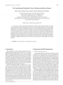
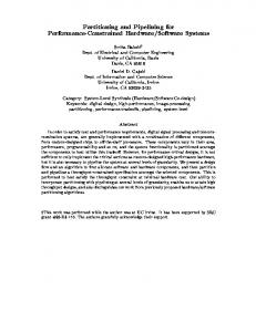
To evaluate our energy optimization techniques, we experiment with mapping the ATR algorithm onto two fixed partitioning schemes: (a) a single-node that combines all blocks, and (b) a five-node pipeline that maps each block onto an individual node (Fig. 6). The input data size is 128K bits, and the output is 14K bits per frame. In scheme (a), the single node combines all the workload of five nodes in (b); and it eliminates all internal communication instances between nodes in (b). (a) and (b) are two extremes representing serial vs. parallel schemes. For both (a) and (b) we apply optimal speed selection. We also find the optimal partitioning with speed selection as (c) and compare its energy consumption with (a) and (b) under two types of performance requirements: (1) high performance, D = 10ms, (2) moderate performance, D = 15ms. Each node consists of an Intel XScale processor [2] whose power vs. performance level ranges from 50mW@150MHz to 1.6W@1GHz (Fig. 7), and an Intel LXT-1000 Ethernet interface [1] with power levels of 0.8W@10Mbps, 1.5W@100Mbps, and 6W@1000Mbps (Fig. 8). We assume each node has a constant power draw Povh = 100mW . The results are presented in Fig. 9. In all cases, 1000Mbps is always the optimal speed setting for communication. The low-power, 10Mbps communication speed results in the highest energy. This is because it leaves so little time for computation such that the processors must run faster with more energy to meet the deadline, and it has the highest energy-per-bit rating. The low-speed communication also tends to violate the schedulability conditions [8]. Given properties of this particular Ethernet interface, 1000Mbps communication will always lead to the lowest energy consumption since it requires the least amount of energy per bit and leaves the maximum amount of time budget for reducing CPU energy. However, in cases where the energy-per-bit rating does not decrease monotonically with the communication speed, the optimal speed setting may involve some combinations of low-speed and high-speed settings between different nodes. For example, the node Ni may communicate with Ni−1 at 1000Mbps and with Ni+1 at 100Mbps. Fig 9(1) shows the energy consumption of all three partitioning schemes under a tight performance constraint. The single-node (a) is heavily loaded with computation. Therefore it is desirable to reduce CPU energy by pipelining. As a result, the five-node pipeline (b) is more energy-efficient at the cost of additional communication and overhead. However, the optimal partitioning is (c) with three nodes: [N1, N2], [N3, N4], [N5]. It consumes more CPU energy than (b), but overall it is optimal with less energy on communication and overhead. In case of the moderate performance constraint (Fig 9(2)), (a) is still dominated by computation but it is not heavily loaded due to

tation compete over opportunities for operating at the most energyefficient points. It is critical to not only balance the load among processors by functional partitioning, but also to balance the speeds between communication and computation on each node and across the whole system. Our multi-dimensional dynamic programming formulation is exact and produces the energy-optimal solution as defined by a partitioning scheme and the speed selections for all computation and communication tasks. We expect this technique to be applicable to a large class of data dominated systems that can be structured in a pipelined organization.

8.

Figure 7: Power vs. performance of the XScale processor. Mode

Power consumption

10M bps

800 mW

100M bps

1.5W

1000M bps

6W

Energy (mJ)

Figure 8: Power modes of the Ethernet interface. 14

14

12

12

10

10

8

8

6

6

4

4

2

2

0

0

(a) 1-node

(b) 5-node (c) Optimal N1N2 | N3 N4 | N5

(1) high performance D = 10ms Overhead

(a) 1-node

(b) 5-node (c) Optimal N1N2N3N4 | N5

(2) moderate performance D = 15ms

Communication

Computation

Figure 9: Experiment results.

the relaxed deadline. The reduction of CPU energy by (b) cannot compensate for the added overhead of new nodes and communication. Therefore (a) is better than (b) and pipelining seems inefficient. However, the optimal partitioning (c) is still a pipelined solution. It combines N1, N2, N3, N4 into one node and maps N5 to another node. (c) achieves minimum energy by appropriately balancing computation, communication with pipelining overhead. If the performance constraint is further relaxed, the serial solution (a) will become optimal.

7.

CONCLUSION

We present an energy optimization technique for networked embedded processors and emerging system-on-chip architectures with high-speed on-chip networks. We exploit with the multi-speed feature of modern high-speed communication interfaces as an effective way to complement and enhance today’s CPU-centric power optimization approaches. In such systems, communication and compu-

REFERENCES

[1] INTEL ethernet PHYs/transceivers. http://developer.intel.com/design/network/products/ ethernet/linecard ept.htm. [2] INTEL XScale microarchitecture. http://developer.intel.com/design/intelxscale/. [3] N. K. Bambha, S. S. Bhattacharyya, J. Teich, and E. Zitzler. Hybrid global/local search strategies for dynamic voltage scaling in embedded multiprocessors. In Proc. International Symposium on Hardware/Software Codesign, pages 243–248, 2001. [4] R. Cherabuddi, M. Bayoumi, and H. Krishnamurthy. A low power based system partitioning and binding technique for multi-chip module architectures. In Proc. Great Lakes Symposium on VLSI, pages 156–162, 1997. [5] P. Eles, A. Doboli, P. Pop, and Z. Peng. Scheduling with bus access optimization for distributed embedded systems. IEEE Transactions on VLSI Systems, 8(5):472–491, 2000. [6] E. Huwang, F. Vahid, and Y.-C. Hsu. FSMD functional partitioning for low power. In Proc. Design, Automation and Test in Europe, pages 22–28, 1999. [7] P. V. Knudsen and J. Madsen. Integrating communication protocol selection with hardware/software codesign. IEEE Transactions on Computer-Aided Design of Integrated Circuits and Systems, 18(8):1077–1095, August 1999. [8] J. Liu, P. H. Chou, and N. Bagherzadeh. Communication speed selection for embedded systems with networked voltage-scalable processors. In Proc. International Symposium on Hardware/Software Codesign, pages 169–174, April 2002. [9] J. Luo and N. K. Jha. Battery-aware static scheduling for distributed real-time embedded systems. In Proc. Design Automation Conference, pages 444–449, June 2001. [10] R. Ortega and G. Borriello. Communication synthesis for distributed embedded systems. In Proc. International Conference on Computer-Aided Design, pages 437–444, 1998. [11] A. Wang and A. Chandrakasan. Energy efficient system partitioning for distributed wireless sensor networks. In Proc. IEEE International Conference on Acoustics, Speech and Signal Processing, pages 905–908, May 2001. [12] E. F. Weglarz, K. K. Saluja, and M. H. Lipasti. Minimizing energy consumption for high-performance processing. In Proc. Asian and South Pacific Design Automation Conference, pages 199–204, 2002. [13] W. Wolf. An architectural co-synthesis algorithm for distributed embedded computing systems. IEEE Transactions on VLSI Systems, pages 218–229, June 1997.