Sarin 1985; Hazen 1986; Salo and Hämäläinen 1992,. 2001; Mustajoki et al. 2005; Salo and Punkka 2005;. Liesiö et al. 2007, 2008). We believe that our model, ...
Decision Analysis
informs
Vol. 6, No. 3, September 2009, pp. 139–152 issn 1545-8490 � eissn 1545-8504 � 09 � 0603 � 0139
®
doi 10.1287/deca.1090.0143 © 2009 INFORMS
Combining a Multiattribute Value Function with an Optimization Model: An Application to Dynamic Resource Allocation for Infrastructure Maintenance Pekka Mild
Systems Analysis Laboratory, Helsinki University of Technology, 02015 TKK, Finland; and Pöyry Infra Ltd., 01621 Vantaa, Finland, pekka.mild@tkk.fi
Ahti Salo
Systems Analysis Laboratory, Helsinki University of Technology, 02015 TKK, Finland, ahti.salo@tkk.fi
A
key decision in infrastructure management is the allocation of resources to maintenance activities that consist of periodic rehabilitation actions and routine day-to-day operations. These activities improve the quality of different assets and operations. They also differ in terms of their objectives, costs, and life-cycle characteristics; yet they all impact the same infrastructure system and compete for resources from the same budget. To support the allocation of resources to these activities, we present a generic resource allocation model that we developed for the Finnish Road Administration (Finnra) by building and interlinking (i) a preference model, which yields the aggregate value of maintenance activities by applying multiattribute value functions to the quality distributions of assets; (ii) a life-cycle model, which captures the deterioration-improvement dynamics associated with the maintenance activities; and (iii) an optimization model, which generates funding recommendations for maximizing the aggregate long-term value of maintenance investments. The optimization results were explored in facilitated workshops where “on-the-fly” computations gave senior managers insights into how the recommendations depended on preferences and budget levels. The case study was awarded for an outstanding achievement in Finnra’s research program, and it was also recognized as a Finalist for the Decision Analysis Society Practice Award in 2007. Key words: decision analysis; OR practice; multiple criteria; resource allocation History: Received on November 4, 2008. Accepted on March 4, 2009, after 1 revision. Published online in Articles in Advance May 21, 2009.
1.
Introduction
infrastructure budgets (see, e.g., Organisation for Economic Co-operation and Development 2008). In broad terms, planning decisions in the maintenance of transportation infrastructures are taken (i) at the programming level, where the focus is on the life-cycle analysis of individual assets and, more specifically, the selection of those actions that will be funded through annual maintenance and repair programs with preestablished budgets; and (ii) at the network level, where the focus is on the aggregate quality distributions of assets and services, and the purpose is to guide the allocation of resources among different maintenance activities, infrastructure asset types, road districts, or other subnetworks. These network-level decisions are inherently more strategic because they set the budgets for the optimization
The construction and maintenance of transportation infrastructures—such as road and rail networks— have long-term impacts on the environment and the competitiveness of industries, as well as social and regional development, among others. These infrastructures also call for major investments, because in industrialized nations their book value can be several percentage points of the gross domestic product. Whereas the construction of new infrastructures tends to attract most public attention, the maintenance and operation of existing infrastructures often consume more resources and have broader long-term impacts. In countries with fully developed transportation infrastructures, for instance, maintenance activities can consume as much as 60%–70% of 139
140
Mild and Salo: Combining a Multiattribute Value Function with an Optimization Model
of programming-level decisions. From the viewpoint of decision support, network-level decisions are also more challenging because they must address longer time horizons and a broader range of objectives. In effect, they are essential to the sustainable development of the whole network. In the context of road networks, maintenance management can be organized as a hierarchy of activities that belong to two main categories: (i) periodic rehabilitation and (ii) routine operations. Periodic rehabilitation actions restore or improve the condition of deteriorating physical assets (e.g., pavements, bridges, gravel roads, and road equipment), whereas routine operations seek to secure the day-to-day trafficability of the road network (e.g., wintertime plowing and deicing, minor repairs and maintenance of road surroundings, gravel roads surface treatments). The activities within and between the two categories differ from each other in terms of their costs and the durability of their impacts, but they all contribute to the overall service level of the same road system and compete for resources from the same budget. As a result, there is a need for systematic and transparent decision support tools that permit trade-offs among multiple objectives and integrate analyses across several assets and operations (National Cooperative Highway Research Program 2005, Krugler et al. 2007). Motivated by this need, we present an integrated decision model for the allocation of resources to different maintenance activities. This model—which is quite generic even though it was initially developed for the Finnish Road Administration (Finnra)— consists of (i) a multicriteria model for determining the value of quality distributions associated with maintenance activities; (ii) a life-cycle model for describing the dynamics of quality distributions (i.e., deterioration of asset quality over time, improvement of asset quality due to maintenance); and (iii) an optimization model for maximizing the long-term aggregate value of all activities through dynamic funding allocations, subject to annual budgets, quality targets, and other constraints. During model deployment, we also conducted extensive sensitivity analyses, incorporated ordinal preference statements about the relative importance of the criteria, and explored the implications of these statements for recommended resource allocations (cf. Kirkwood and
Decision Analysis 6(3), pp. 139–152, © 2009 INFORMS
Sarin 1985; Hazen 1986; Salo and Hämäläinen 1992, 2001; Mustajoki et al. 2005; Salo and Punkka 2005; Liesiö et al. 2007, 2008). We believe that our model, its enthusiastic uptake by senior managers, and subsequent development efforts at Finnra are one of the first successful attempts at integrated resource planning for road maintenance activities. One plausible reason for this was that this model was built on existing data and formulated at a relatively high level of aggregation; therefore, it was transparent enough to support interactive analyses in facilitated workshops (instead of offering seemingly “optimal” take-it-or-leave-it recommendations). These workshops allowed the managers to engage in exploratory, evidence-based discussions about the funding levels that are required in the long term (cf., e.g., Peerenboom et al. 1989, Gamvros et al. 2006, Kleinmuntz 2007, Phillips 2007). The managers were particularly interested in exploring (i) how much funding should be given to different activities when considering these activities jointly without the constraints of prior budgeting practices, (ii) how the recommended funding levels would change in response to different preference statements, and (iii) how possible changes in the total level of funding would be reflected in funding priorities. The possibility to address “softer” criteria explicitly—such as customer satisfaction—was helpful, too, because it highlighted what maintenance activities contributed most to the attainment of these criteria, and how funding levels should be adjusted to account for them. The rest of this paper is structured as follows. Section 2 discusses earlier models for infrastructure management and describes the context for our case study at the Finnish Road Administration. Section 3 presents the integrated resource allocation model. Section 4 describes its key results and sensitivity analyses, and discusses how they were explored in interactive workshops. Section 5 outlines extensions for future research and development. Section 6 concludes.
2.
Background and Objectives
2.1. Challenges in Integrated Resource Allocation Since the 1980s, transportation agencies in countries like the United States, United Kingdom, Australia, Germany, and Finland have developed network-level models to predict how the quality distributions of
Mild and Salo: Combining a Multiattribute Value Function with an Optimization Model Decision Analysis 6(3), pp. 139–152, © 2009 INFORMS
infrastructure assets will evolve in response to maintenance decisions (Golabi et al. 1982, Golabi and Shepard 1997). Most of these employ Markov decision processes (MDPs) that describe the stochastic evolution of the assets’ quality levels based on empirical data about deterioration rates and the impacts of preventive/corrective rehabilitation actions. These actions incur costs to the transportation agency, whereas the lower asset quality incurs greater costs to the users (e.g., greater risk of accidents, increased travel time, higher fuel consumption). The MDP models seek to minimize the total socioeconomic sum of all of these costs subject to quality constraints. Their solutions are derived from the steady state of the Markov chain, and they also show the most cost-effective path for reaching this state. These results support long-term budgeting by characterizing optimal funding levels for rehabilitation actions, and by conveying the corresponding distributions of asset quality. Although technically and economically sound, cost minimization models have several deficiencies from the viewpoint of integrated resource planning: • The MDP models usually focus on the pavements and bridges of the primary road network, which has a high traffic volume and which is usually best understood and also most effectively managed. However, these models are often quite complex, which makes it difficult to calibrate their parameters and communicate their assumptions. For example, their cost parameters and quality constraints may relate to multiple objectives in complex and nontransparent ways; therefore, they are not ideal for explorative interactive analyses. • Quality-dependent user costs may not exist for all assets and activities, particularly for routine operations or rehabilitation actions on the secondary road network with a lower traffic volume. Furthermore, routine operations are inherently different from rehabilitation actions in terms of their deterioration characteristics. Such differences among activities undermine possibilities of using existing cost-based model structures for between-activity comparisons. • Increasing pressures toward the explicit recognition of multiple objectives in infrastructure management (e.g., increased safety, higher customer satisfaction, reduced environmental impacts) make it necessary to address impact dimensions beyond
141
cost considerations (e.g., Kulkarni et al. 2004, National Cooperative Highway Research Program 2005). Because many of these objectives—such as customer satisfaction—are inherently subjective, there is a need for approaches that accommodate preferences explicitly. In view of these considerations, cost-based MDP models are not really adequate for comprehensive analyses where the managers must address the shortand long-term impacts of different activities with regard to multiple objectives. This creates a need for integrated approaches that capture these multiple objectives, the decision makers’ subjective preferences, and also the life-cycle dynamics of infrastructure assets, with the aim of supporting the allocation of resources to different activities. 2.2. Finnish Road Administration (Finnra) Finnra is responsible for the management of the Finnish public road network, which has an asset value of 15 billion euros and comprises 78,000 kilometers (km) of roads and 14,000 bridges. Finnra’s annual turnover is about 600 million euros, of which some 400 million euros is spent on maintenance. Because of geographical reasons, the Finnish road network has some unique characteristics such as (i) an extensive active gravel road network of 23,000 km that must be maintained even at low traffic volumes, and (ii) snowy and icy conditions that call for routine wintertime operations during three to six months per year. These characteristics, however, do not limit the relevance of our resource allocation model for other countries, states, or regions. Finnra has a central administration and nine road districts. The central administration allocates annual budgets to the districts and sets performance targets to enforce national policies. The road districts manage infrastructure assets in their regions by developing annual maintenance plans and by implementing these plans by acquiring services from contractors through competitive tendering. Although the central administration sets strict budgets and performance targets, each district has some autonomy in adjusting national guidelines according to its needs. In the districts, different maintenance activities have their own managers and designated experts with partly overlapping domains of expertise. The managers work in close collaboration but also compete for resources.
Mild and Salo: Combining a Multiattribute Value Function with an Optimization Model
142
Decision Analysis 6(3), pp. 139–152, © 2009 INFORMS
Our resource allocation model was developed for the road district of Southeastern Finland in 2006. Its development was motivated by the question of what changes would be called for in the current allocation of resources to different activities if there were alternative assumptions about the relevance of the impact criteria. It was conjectured that decision analytic modeling could be useful in this context, all the more so due to positive experiences from our earlier collaboration with Finnra on the use of robust portfolio modeling (Liesiö et al. 2007, 2008) in the development of bridge repair programs. The project team consisted of the authors of this paper, a senior manager from Finnra’s central administration, a senior consultant from Pöyry Infra, and three maintenance managers from the Southeast Finland road district. The development of the value model involved five further experts, and the workshops for the dissemination of results were attended by senior managers from the road district, including its general director and financial director. The project involved some 10 man-months of work and lasted about 8 months. Requisite data were obtained either from Finnra’s databases (e.g., asset volumes, initial quality distributions) or estimated by experts in facilitated workshops. Standard software tools were employed to develop tools for preference elicitation (Microsoft Excel® ) and the computation and visualizations of results (Matlab® , Xpress-MP® ).
3.
Integrated Multicriteria Model
3.1. Maintenance Activities and Quality Classes The activity structure in Figure 1 was derived from Finnra’s standardized definitions with the aim of balFigure 1
ancing decision support needs with modeling issues (e.g., appropriate level of detail, data availability, required preference elicitation efforts). Of the seven main activities, four were periodic rehabilitation actions, and three were routine operations. Where appropriate, the main activities were divided further, for instance, by regarding actions on pavements with high and low traffic volumes as two separate activities; this resulted in a total of 13 twig-level activities in need of resources. For each activity, five quality classes were defined to characterize different service levels. As in most network-level analyses, the activities were analyzed by considering the distribution of total asset volume across quality classes (i.e., the quality distribution). This volume was expressed in terms of basic asset units, either by counting individual items (bridges) or summing one-kilometer segments of roads (all other activities). Specifically, for each activity, the quality distribution indicated what the volume of corresponding assets in the five quality classes was (e.g., 1,400 bridges in condition quality class 1, or 1,500 kilometers of high-traffic-volume roads maintained in routine operations quality class 5). The definitions of the quality classes were taken directly from Finnra’s standardized classifications with predefined thresholds on technical condition parameters and service specifications. These classifications had been developed earlier to establish a unified scheme where the same class descriptors represented comparable service levels across different activities. This operationalization of quality classes ensured that (i) each asset unit belonged to exactly one quality class at any given time, (ii) the extreme classes represented the worst and best plausible
Activity Structure Consisting of 13 Activities with Five Quality Classes for Each
Road district’s annual maintenance budget
Periodic rehabilitation
Pavements High traffic Low 1 2 3 4 5
Bridges
Gravel roads
Routine operations Road equipment
Wintertime
Road surroundings
Gravel roads
Mild and Salo: Combining a Multiattribute Value Function with an Optimization Model
143
Decision Analysis 6(3), pp. 139–152, © 2009 INFORMS
service levels, and (iii) differences between quality classes were significant enough to be operationally meaningful in terms of their impacts and technical parameters (e.g., costs). Of the 13 activities, only routine operations on road surroundings and gravel roads did not have previously established quality classes. We constructed the classes for these by taking the service level achieved by the current funding level as the midpoint quality and considering funding levels at ±10% and ±20% to define two inferior �−10%� −20%� and two superior �+10%� +20%� quality classes. These changes in funding levels complied with the requirements (i)–(iii) above and resulted in classifications that were sufficiently comparable to the standardized ones already developed for other purposes. For the classes that were thus constructed, Finnra’s experts also specified the corresponding physical service levels, which gave enough technical information for the assessment of their impacts. Overall, we thus had five well-defined quality classes for each of the 13 activities and corresponding initial quality distributions that represented the status quo of the road district. The initial distributions were obtained from Finnra’s data records, which are updated annually based on condition measurements, latest actions, and operational contracts. Within each quality class, the asset units represented the “average” characteristics of the actual physical units assigned to the class. From the modeling point of view, this meant that the same (average) parameter values were applied to the total number of asset units that were assigned to a particular quality class for a particular activity. In principle, the activities could have been decomposed further (e.g., based on subnetworks with different traffic volumes) to achieve greater model resolution and more homogenous classes of actual asset units. Such added detail would not have changed the model structure, but it would have resulted in a larger model and called for greater elicitation efforts. On this point, Finnra’s experts judged that the structure in Figure 1 was sufficiently detailed, particularly in view of the objective of analyzing all activities jointly. 3.2. Multicriteria Evaluation Model To support comparisons of different quality distributions within and between the activities with regard
Table 1
Four Evaluation Criteria for Quality Classes
Criterion Road safety Asset value preservation Customer satisfaction
Environmental aspects
Brief description Frequency and severity of road accidents due to poor quality of assets and routine operations. Monetary decline in asset value (cf. increase in maintenance and repair costs) due to deterioration of asset quality. Service level as perceived by road users in terms of driving comfort, sustained driving speed, and safety confidence; customer feedback. Adverse effects of road chemicals, traffic noise, and dusting; aspects of nature conservation, tidiness, and appearance.
to multiple criteria over a multiyear time horizon, we built a weighted-additive value function based on multiattribute value theory (see, e.g., Keeney and Raiffa 1976, Kirkwood 1997). The quality distributions were evaluated with regard to the four criteria (see Table 1) that were derived from Finnra’s formal mission statement. Apart from descriptive titles, detailed descriptions were developed based on discussions with Finnra’s experts to ensure that these criteria would be interpreted consistently throughout model development and its use. The overall additive value function was aggregated from the evaluation of activity × quality class × year—combinations characterized by numbers of asset units that would belong to a given quality class at a given year of the planning horizon (i.e., 13 × 5 = 65 activity × quality class combinations, 65 × 50 = 3�250 activity × quality class × year combinations). The decision recommendations consisted of funding levels that would impact the number of assets in these quality classes over the planning horizon, based on the costs and impacts of maintenance activities as well as the deterioration dynamics of asset quality. More formally, the subscripts/superscripts of t = 1� � � � � 50 refer to the years of the planning horizon, i = 1� � � � � 13 to the maintenance activities, j = 1� � � � � 5 to different quality classes, and k = 1� � � � � 4 to the evaluation criteria. Moreover, aij �t� denotes the number of asset units of activity i in quality class j in year t. The structure of the value model was as follows: � �13 �5 i i 1. The overall value V = 50 t=1 i=1 j=1 vj� t �aj �t�� was formed as the sum of values vj�i t �aij �t�� associated
Mild and Salo: Combining a Multiattribute Value Function with an Optimization Model
144
Decision Analysis 6(3), pp. 139–152, © 2009 INFORMS
with having aij �t� asset units of activity i in quality class j at year t. 2. The value vj�i t �aij �t�� was assumed to be linear so that it could be expressed by multiplying aij �t�, the number of asset units of activity i in quality class j, by vji , the value of a single asset unit of activity i in quality class j. The future values were weighted by a discount factor dt = �1 + r�−t with a discount rate r = 3% (subsequent sensitivity analyses showed that the optimization results were quite robust with regard to the discount rate). Thus, vj�i t �aij �t�� = dt vji aij �t�. 3. The four evaluation criteria in Table 1 were used to determine vji through an additive weighted � value function, vji = 4k=1 wk wki vj�i k , where vj�i k was the single-criterion value score of quality class j for activity i under criterion k, wki was the relative weight of activity i under criterion k, and wk was the weight of the criterion k. 4. Based on the above decomposition, the overall value could be written as V =
5 � 4 13 � 50 � � t=1 i=1 j=1 k=1
=
50 � t=1
dt
5 13 � � i=1 j=1
dt wk wki vj�i k aij �t�
aij �t�
4 � k=1
wk wki vj�i k �
The single-criterion value functions vj�i k were elicited over the five quality classes (j = 1� � � � � 5) for each of the 13 activities �i = 1� � � � � 13� for the four criteria �k = 1� � � � � 4�. The worst and best quality classes for each activity and criterion were assigned scores i i v1� k = 0 and v5� k = 100, respectively. The intermediate quality classes were evaluated with respect to these extreme classes and, for the purposes of validation, also with respect to each other. The elicitation questions started by encouraging the respondents to state their ordinal preferences for quality differences (e.g., is the quality difference between classes 3 and 4 more or less significant than that between quality classes 2 and 3). The responses were recorded into an Excel® tool and they were validated and adjusted through visual inspection as well. This approach assigned a cardinal score vj�i k in the range of 0–100 to each quality class. (See Figure 2, which contains some illustrative data. The double-headed arrows highlight which points of the value function were being adjusted.)
Figure 2
Within-Activity Value Function for Activity i with Regard to Criterion k (Determination of Intermediate Scores)
Score vj�i k
Criterion k
100
Product i
50
0 1
2
3
4
5
Class j
For each criterion, the activity weights wki �i = 1� � � � � 13� were elicited by comparing the greatest quality improvements (“swings”) that were associated with different maintenance activities. Specifically, we applied SWING-weighting (von Winterfeldt and Edwards 1986) by assigning an activity weight wki = 1 to the activity for which the impact of quality improvement (per asset unit) from quality class 1 to class 5 was considered greater than that for any other activity. The activity weights for the other activities were estimated by comparing the significance of their respective 1-to-5 quality swings in relation to this maximum swing, and by setting the corresponding activity weight wki accordingly in the range from 0 to 1. Throughout the elicitation of these activity weights, the shapes of the value functions obtained from score elicitation were displayed to the respondents (Figure 3). For each activity, the elicited value scores and the activity weights established criterionspecific value functions wki vj�k k that could be applied to the corresponding quality distribution. The criterion weight wk reflected the value increase that would have been obtained by moving a single asset unit of the activity with the highest activity weight under criterion k from the worst quality class to the best quality class. These weights guided the prioritization of activities; for example, as a result of increasing the weight wk , the value of such major quality improvements would have been grown more for activities with high activity weights, and thus the value–cost ratio of these activities would have improved as well. At the extreme, if all the weight had
Mild and Salo: Combining a Multiattribute Value Function with an Optimization Model Decision Analysis 6(3), pp. 139–152, © 2009 INFORMS
Figure 3
Between-Activity Evaluation of Activities with Regard to Criterion k (Determination of Activity Weights wki from the Consideration of Maximum Swings)
Value wki vj�i k
Criterion k
100 Product i +1 Product i 50 Product i –1 0 1
2
3
4
5
Class j
been assigned to a single criterion, only those scores and activity weights that pertained to this criterion would have mattered in the overall value function. To study the impacts of different criterion preferences, we explored uses of incomplete information through preference programming methods (Kirkwood and Sarin 1985; Hazen 1986; Salo and Hämäläinen 1992, 2001; Mustajoki et al. 2005; Salo and Punkka 2005; Liesiö et al. 2007, 2008) so that, instead of focusing on a single vector of criterion weights, we considered a feasible weight set that was consistent with ordinal preference statements about the relative importance of the criteria. This set was derived from an incomplete rank ordering provided by Finnra’s experts (cf. Salo and Punkka 2005), who noted that road safety and asset value preservation were the two most important criteria (without specifying which one would be the most important), followed by customer satisfaction as the third, and environmental aspects as the fourth most important criterion. 3.3. Life-Cycle Dynamics and Optimization The quality of assets deteriorates over time due to traffic and environmental loads. In terms of quality distributions, this implies that asset units in the higher quality classes fall to the lower quality classes unless actions are taken to raise them back to the higher classes. For routine operations, quality distributions are determined directly by the volumes of assets maintained according to the service specifications of the different quality classes. Thus, the quality distributions evolve dynamically over time (in
145
one-year time steps) as a function of annual maintenance decisions. In our optimization model, decision variables for rehabilitation actions corresponded to decisions about how many asset units in quality class j should be raised to some higher quality class j � > j in a given year t. For routine operations, they corresponded to decisions about how many asset units should be held in quality class j in a given year t. To capture the deterioration-improvement dynamics, we built a simple life-cycle model based on established Markovian principles (cf. Golabi et al. 1982, Golabi and Shepard 1997). For all rehabilitation activities, a fixed percentage of the share of assets in a given quality class was assumed to fall to the quality class immediately below it in one year’s time. Where appropriate, these activity- and class-specific percentages were estimated using evidence about deterioration times and average lifecycles of assets and actions. The class-specific unit cost of raising assets from a lower to higher class was estimated based on past records and expert judgments. For routine operations, the decisions defined the quality distribution for each year, and hence no deterioration models were needed. The unit cost of routine operations in different quality classes was derived from existing service contracts or estimated through expert judgments using quality class definitions. In general, the activities exhibited quite different cost characteristics and service lives. For instance, the unit costs of the actions varied from a few hundred euros to several hundreds of thousands of euros, and the improved service levels could be sustained anywhere between 1 to 30 years. The time span of the model was set to 50 years, which was long enough to cover the full dynamics of all activities and actions taken in the later years of the model run. The multicriteria value model and life-cycle dynamics model were combined into an optimization model that yielded dynamic resource allocation recommendations for the funding of different activities. The objective function of this linear programming model was the discounted sum of the annual aggregate values of the activities’ quality distributions as presented in §3.2. It was maximized by allocating funds to rehabilitation actions and routine operations.
Mild and Salo: Combining a Multiattribute Value Function with an Optimization Model
146
Figure 4
Decision Analysis 6(3), pp. 139–152, © 2009 INFORMS
Change of Value from Year t to t + n for the Quality Distribution of Activity i
Quality distribution at time t
Quality distribution at time t + n
i j
a �t�
Time deteriorates
Funding improves 1
2
3
4
5
Road safety
1
Asset value
2
Customer
3
4
5
Environment
wki vj�i k
1
2
V i �t� =
3
� j
4
aij �t�
5
�
1
2
3
4
5
1
2
3
4
5
1
2
3
4
5
wk wki vj�i k annual overall value of the quality distribution
k
V i �t�
Environment Customer Asset value Road safety
t+n
t
The Markov-chain-based deterioration-improvement dynamics were captured through linear constraints. Additional constraints were introduced to capture budget limitations and threshold requirements on quality distributions. The principle of associating multicriteria value with a dynamically developing quality distribution is illustrated in Figure 4. Specifically, the quality distribution changes over time due to deterioration, on one hand, and funded quality improvements, on the other hand. The multicriteria value function associates an overall value with the quality distribution each year, and this value changes when the quality distribution changes. The dynamic development of this value can thus be controlled through resource allocation decisions. The complete model is presented in the appendix.
4. 4.1.
Model Results and Sensitivity Analyses
Decision Recommendations and Management Insights The optimization yielded “funding curves” that conveyed how much funding should be allocated to each activity on a year-to-year basis. These recommended resource allocations were computed with and without activity-specific budget constraints. Without these constraints, the recommendations suggested some unrealistically large departures from the status quo, and therefore further analyses were carried out by setting upper and lower bounds on the funding levels that could be meaningfully allocated to the activities. These bounds were derived from the supply capabilities of market contractors, and they prevented excessively large and sharp devia-
Mild and Salo: Combining a Multiattribute Value Function with an Optimization Model
147
Decision Analysis 6(3), pp. 139–152, © 2009 INFORMS
Figure 5
Base-Case Funding Curves for Total Annual Funding of 40 Million Euros 14 Pavements (rehab)
13
Wintertime (routine)
12
Funding allocated to product (MF)
11 10 9
Computed average funding 8 7
Road surroundings (routine)
6 5
Gravel roads (routine)
4
Bridges (rehab)
3 2
Gravel roads (rehab)
1
Road equipment (rehab)
2030
2029
2028
2027
2026
2025
2024
2023
2022
2021
2020
2019
2018
2017
2016
2015
2014
2013
2012
2011
2010
2009
2008
2007
2006
0
Year
tions from the initial funding levels. They also helped ensure that all activities would fulfill their respective minimum quality requirements. Once these minimum requirements were fulfilled, the model could be used to explore possibilities for further improvements (cf., e.g., Kleinmuntz 2007). In the base-case solution, incomplete preference information about the importance of the criteria was explored by using Monte Carlo sampling to generate criterion weights that complied with the ordinal preference statements (i.e., road safety and asset value preservation as the two most important criteria, followed by customer satisfaction and, finally, environmental aspects). The base-case solution in Figure 5 was obtained by generating 1,000 criterion weights and by averaging the corresponding optimal funding solutions on a year-by-year basis. In addition, the solutions that corresponded to the extreme points of the feasible weight set were examined in detail. The recommended funding levels for the activities were aggregated to show the funding curves for the seven main activities in Figure 1, because Finnra was most interested in the comparison of these activities. For visualization purposes, the funding curves were smoothed by computing three-year moving averages,
further to the recognition that abrupt changes would be undesirable because the contractors were unable to build up new service capacity very quickly, nor did they wish to experience sudden reductions in the demand for their services. The base-case solution supported several important conclusions that also exemplify what kinds of results integrated resource allocation models can offer: • Maintenance backlog of bridges. The funding curve for the rehabilitation of bridges indicated that there was a need for rapid corrective actions to improve the relatively poor status quo quality of bridges. This need had already been recognized in national policies and it was not, therefore, particularly surprising; however, it was validated by the model, which thus provided additional justification for a shift in funding policies. • Dynamic funding patterns. The detailed analysis showed that the funding curves for the different activities were inherently dynamic so that the relative shares of funding allocated to different activities should change over time to respond to the needs of the different activities. This was an important finding because it differed markedly from earlier funding policies where the different activities had had rela-
148
Mild and Salo: Combining a Multiattribute Value Function with an Optimization Model
tively rigid and static shares of the overall budget from year to year. • Impacts on customer satisfaction. For example, the model suggested that increased funding should be given to routine operations, because these tend to have a strong impact on customer satisfaction. The link had been implicitly recognized, but the model provided an analytical justification for how increased emphasis on customer satisfaction (interpreted in terms of a higher criterion weight) would be reflected in funding levels. Likewise, the model highlighted that improving the quality of road equipment (e.g., road markings, signs, guardrails) would indeed be a relatively inexpensive way to increase customer satisfaction. The model results were communicated in an interactive facilitated workshop, which was attended by the managers of the Southeast Finland road district. In this workshop, the focus was on the funding curves and their corresponding quality distributions, and therefore most attention was given to the dynamic behavior and relative magnitudes of funding curves. Specifically, the managers could pose questions about how the funding levels would be affected by different preferences or changing quality requirements. These questions were addressed by changing the model parameters, by computing the results “on the fly,” and by presenting the revised results in a minute or less. This mode of truly interactive model-based analysis was a totally new way of working at Finnra. In particular, the ability to consider all activities simultaneously provided fresh insights and catalyzed discussions about required policy changes. 4.2. Exploration of Criterion Weights We also conducted extensive sensitivity analyses with regard to criterion weights, based on preference statements about the importance of the four criteria. In particular, we examined (i) minimum and maximum bounds on funding levels, determined for each year as the minimum and maximum level of funding proposed by the funding curves that corresponded to the 1,000 sampled weight vectors; and (ii) the extreme funding curves, which corresponded to the extreme points of the feasible weight set. The lower and upper bounds from sampled weights indicated which activities were most sensitive to criterion weights. Activities with wide bounds
Decision Analysis 6(3), pp. 139–152, © 2009 INFORMS
tended to perform well only on one or two criteria and were hence more sensitive to weights. Activities with more robust funding curves (in terms of relatively tight bounds around the base-case solution) performed relatively well on most criteria and/or exhibited high benefit–cost ratios (i.e., although the value of some activities was sensitive to criterion weights, they had low enough costs to offer better value–cost ratios than other activities). The extreme funding curves showed how the activities would be prioritized as a function of different criterion weights. To some extent, this prioritization might have been deduced from the evaluation scores, but the funding curves were backed up by more evidence because they also accounted for the initial quality distributions, deterioration-improvement dynamics, and costs of maintenance activities. The funding curves for weight vectors where some criteria did not have any weight tended to be volatile and infeasible for practical implementation; nevertheless, they were useful for validation purposes and for catalyzing discussions. Overall, the exploration of different criterion weights was very instructive. Indeed, our experiences from the workshop suggest that it may be beneficial to conduct such analyses in a truly explorative manner, instead of first computing the “optimal” solution followed by limited sensitivity analyses on selected model parameters, although the numerical results from the two approaches may not differ considerably. In our case study, the exploration of incomplete information was much appreciated by the managers because it helped them understand why the results looked the way they did. This, we believe, made it easier for them to accept the model and its results. 4.3. Changing Budget Levels The model was also used to analyze how the prioritization of activities would change in response to changes in the overall budget. Specifically, because the budgets are expected to be on the decline, we explored how cuts in the budget, introduced at consecutive steps of 5% reductions, would be reflected in the funding curves of the individual activities. These budget cuts had different implications for different activities, for the funding of some activities was cut dramatically whereas that of others
Mild and Salo: Combining a Multiattribute Value Function with an Optimization Model Decision Analysis 6(3), pp. 139–152, © 2009 INFORMS
remained close to the base-case solution. There were also changes in the temporal patterns of funding levels, because some activities were subjected to cuts during the first few years, but then received increased funding so that the long-term average remained much the same. More generally, our analyses helped establish when and how the activities’ funding level should be changed in response to decreases (or also to increases) in the overall budget. In this context, sensitivity analyses also showed how the resulting priorities depended on the criterion weights. Overall, insights into the prioritization of activities as a function of changing budget levels and criteria weights were among the most significant results. Although much of the annual funding is fixed based on national guidelines, long-term programs, and service contracts, road districts may have to adjust their budgets by ±1%–10% due to needs that arise at a short notice. Toward this end, a prior consensus on activity priorities, achieved through interactive analyses, can be useful for implementing these adjustments. 4.4. Limitations of Linearity Assumptions Our additive formulation assumes that the criteria are mutually preferentially independent. This means, among other things, that the decision maker’s preferences for improving the quality distribution of a maintenance activity with regard to a given criterion does not depend on what the quality distribution of this activity is with regard to the other criteria, or what the quality distributions of the other activities are. Second, the linearity assumption means, for instance, that making a similar quality improvement to the 1st or 1,000th asset unit yields the same value increase. These assumptions may not apply entirely. Yet, when combined with the initial quality distributions, deterioration-improvement dynamics, and other constraints, the model was approved as an adequate approximation for making comparative analyses within a feasible range of variation (cf. Kleinmuntz 2007). Moreover, the optimized results can be extreme in the sense that, for example, if there are 200 km of pavements available for improvement in quality class 1 with a far superior value–cost ratio, then all these pavements will be improved before funds are
149
allocated to quality improvements in other classes and activities. But this does not, however, mean that it would be optimal to move all pavements into quality class 5 before attending to other activities, because 1-to-5 quality improvements of other activities typically yield a higher value increment than the 2-to-5 and 3-to-5 quality improvements of pavements. The specification of constraints was also important in using the model: some actions were enforced to ensure minimum quality while the deterioration dynamics still ensured that the solution space reflected future improvement needs. There are at least three options for extending the model. First, the use of a nonlinear attribute-specific value function, vj�i t �aij �t��, would make it possible to model the decreasing marginal value associated with the growing number of asset units in a quality class. Second, a multiplicative model could be used to capture preference dependencies among the criteria. Although conceptually viable, both options result in more complex models, and neither would allow the use of linear programming solvers. A third option— which would preserve linearity—would be to set aspiration levels on the values that are associated with the activities’ annual quality distributions. The specification of such activity-specific aspiration levels would drive the quality distributions to these levels, but it would not reward unnecessarily for “excessive” quality.
5.
Prospective Extensions
Overall, our pilot model was very well accepted, even though Finnra had not had much prior experience on the deployment of similar decision analytic approaches. First, this model was the first one to help Finnra consider funding priorities among rehabilitation actions and routine operations in an integrated manner. Second, although the model was not very detailed (because it integrated very different types of activities with varying levels of data and modeling detail), it provided a transparent framework that offered valuable management insights and enabled a variety of interactive analyses. In fact, our experiences suggest that the lack of excessive technical detail may make it easier to communicate results and to develop exploratory guidelines about how funding patterns
150
Mild and Salo: Combining a Multiattribute Value Function with an Optimization Model
should be altered in response to shifting preferences or budget changes. At Finnra, our case study has sparked interest in the further development of decision analytic approaches for resource allocation, as evidenced by a larger follow-up project whose objectives illustrate possibilities of extending the model: • The model will be extended to the whole nation to cover all nine road districts. This makes it possible to examine how resources should be allocated among the districts that have different amounts of road infrastructure and different quality distributions as well. Provisional plans have been made to consider investments into the building of new infrastructures along with the maintenance of existing infrastructures. • The model, and also the processes of parameter elicitation and communication of its results, will be revisited to establish a well-defined and repeatable decision support process. Most probably, some parts of the model may undergo major revision, but its main structure is expected to remain the same. • The communication of results will be enhanced by developing “priority maps” that help convey graphically which activities/districts merit increased/ decreased funding when the overall budget is raised/ cut by some percentage points. For example, once the average funding needs for the first 3 and 10 years have been computed, such a map can be presented as a table where the activities and evaluation criteria correspond to rows and columns, respectively, and the cells contain colored symbols that show in what direction and by how much the activity’s funding level should be altered when increased priority is given to some criterion. Such displays summarize many key results from weight-based prioritization of activities. Furthermore, the maintenance of many other infrastructure systems—such as railroads, waterways, and buildings—involve similar questions about how several maintenance activities, multiple criteria, subjective preferences, and deterioration dynamics can best be modeled, often in complex planning environments where complete preference or technical information may be difficult to acquire. It is widely accepted that the exhaustive modeling of these infrastructure systems may not be possible, yet this is not necessary for the purpose of building models that
Decision Analysis 6(3), pp. 139–152, © 2009 INFORMS
serve as validated frameworks in support of structured and repeatable decision-making processes (cf. Peerenboom et al. 1989, Clemen and Kwit 2001, Belton and Stewart 2002, Gamvros et al. 2006, Kleinmuntz 2007, Phillips 2007). It is against this background that we believe that our model is generic enough and would hence be applicable to other infrastructure systems as well.
6.
Conclusions
We have described a case study for the Finnish Road Administration where we developed an integrated decision model for the allocation of resources to maintenance activities. This model—which is generic and, hence, relevant to the maintenance of other infrastructure assets and decision contexts as well—features modules for the evaluation of quality class distributions with regard to multiple criteria, the characterization of deterioration-improvement dynamics of activity quality, and the determination of recommended activity funding levels over a long time horizon. Although some parts of this model were inspired by earlier cost-based models, it is nevertheless quite different because its main purpose is to support the allocation of scarce resources among different activities (rather than to guide the socioeconomically optimal level of spending of resources on any individual maintenance activity). By doing so, it provides strategic decision support to administrators who must continually reprioritize resource allocation levels. The model has allowed Finnra managers to consider multiple criteria, to address trade-offs among these, and to perform extensive sensitivity analyses in facilitated workshops. These interactive workshops with end-user managers have been a crucial part of model deployment because they have allowed the managers to understand, explore, and debate the implications of different modeling assumptions. In effect, these workshops have been “hands-on” learning sessions that have generated important management insights and sparked broader interest in decision analytic modeling activities at Finnra. To quote the closing words of the general director of the Southeast Finland road district at the end of a results workshop, the model and the interactive analyses provided “an innovative and practical platform for thinking
Mild and Salo: Combining a Multiattribute Value Function with an Optimization Model
151
Decision Analysis 6(3), pp. 139–152, © 2009 INFORMS
and communication to support network level strategy work.” Acknowledgments
This research was supported by the Finnish Road Administration and the Academy of Finland. Parts of the paper were written when the second author was working as a visiting professor at the London Business School. The computations were carried out with Xpress-MP© software provided by Dash Optimization Inc. through their Academic Partner Program. The authors thank the three anonymous reviewers for their insightful and constructive comments on this paper.
Appendix A. Resource Allocation Model Index sets REH: Index set of the rehabilitation activities. ROU: Index set of the routine operations activities. Decision variables aij �t�: Number of asset units of activity i in quality class j in year t. i xj� Number of asset units of activity i that are moved j � �t�: from quality class j to quality class j � > j in year t (for rehabilitation actions i ∈ REH). Constants �ij : Percentage of the total number of assets units aij �t� whose quality declines to the next lower quality class in one period (for rehabilitation activities i ∈ REH ). cj�i j � : Cost of raising one asset unit from quality class j to j � > j (for rehabilitation activities i ∈ REH). i cj : Cost of operating one asset unit at the level of quality class j for one year (for routine operations i ∈ ROU ). B�t�: Budget in year t. dt : Annual discount factor calculated from constant rate r as dt = �1 + r�−t . i vj� : Score of activity i for quality class j with regard to k criterion k. wki : Weight of activity i with regard to criterion k. wk : Weight of criterion k drawn from the set of feasible criterion weights Sw , where Sw �= �w = �w1 � � � � � w4 �T � w1 ≥ w3 ≥ w4 � w2 ≥ w3 ≥ w4 � �4 k=1 wk = 1�. �: Upper bound on the share of assets units whose quality level changes from one year to the next. aij �t0 �: Initial number of asset units of activity i quality class j. Constraints The total number of assets units does not change: � � i aj �t� = aij �t0 � ∀ i� t j
j
Moves are nonnegative; the sum of moves from class j cannot exceed the number of assets that are in this class: � i i xj� xj� j � �t� ≤ aij �t� ∀ i� j� j � � t j � �t� ≥ 0� �j � � j � >j�
Deterioration-improvement dynamics: aij �t + 1� = �1 − �ij �aij �t� + �ij+1 aij+1 �t� � i � i xj� j � �t� + xj � � j �t� ∀ i� j� t − j � >j
j �