Syst. Biol. 47(4):568–581, 1998
Combining Data Sets with Different Phylogenetic Histories JOHN J. WIENS Section of Amphibians and Reptiles, Carnegie Museum of Natural History, Pittsburgh, Pennsylvania 15213-4080, USA; E-mail:
[email protected] Abstract.— The possibility that two data sets may have different underlying phylogenetic histories (such as gene trees that deviate from species trees) has become an important argument against combining data in phylogenetic analysis. However, two data sets sampled for a large number of taxa may differ in only part of their histories. This is a realistic scenario and one in which the relative advantages of combined, separate, and consensus analysis become much less clear. I propose a simple methodology for dealing with this situation that involves (1) partitioning the available data to maximize detection of different histories, (2) performing separate analyses of the data sets, and (3) combining the data but considering questionable or unresolved those parts of the combined tree that are strongly contested in the separate analyses (and which therefore may have different histories) until a majority of unlinked data sets support one resolution over another. In support of this methodology, computer simulations suggest that (1) the accuracy of combined analysis for recovering the true species phylogeny may exceed that of either of two separately analyzed data sets under some conditions, particularly when the mismatch between phylogenetic histories is small and the estimates of the underlying histories are imperfect (few characters, high homoplasy, or both) and (2) combined analysis provides a poor estimate of the species tree in areas of the phylogenies with different histories but gives an improved estimate in regions that share the same history. Thus, when there is a localized mismatch between the histories of two data sets, the separate, consensus, and combined analyses may all give unsatisfactory results in certain parts of the phylogeny. Similarly, approaches that allow data combination only after a global test of heterogeneity will suffer from the potential failings of either separate or combined analysis, depending on the outcome of the test. Excision of conicting taxa is also problematic, in that doing so may obfuscate the position of conicting taxa within a larger tree, even when their placement is congruent between data sets. Application of the proposed methodology to molecular and morphological data sets for Sceloporus lizards is discussed. [Combined analysis; computer simulation; consensus analysis; phylogenetic accuracy; Sceloporus; separate analysis.]
A major debate in phylogenetics is whether or not different data sets should be analyzed only separately or should be combined (see reviews by de Queiroz et al., 1995; Miyamoto and Fitch, 1995; Huelsenbeck et al., 1996). An important contribution to this debate has been the idea that different data sets may actually have different underlying phylogenetic topologies (e.g., Doyle, 1992; de Queiroz, 1993; Bull et al., 1993). Differences in phylogenetic histories may be the result of a deviation of the gene tree from the species tree for one or more sets of molecular data, which may be caused by paralogy, lineage sorting of ancestral polymorphisms, or lateral transfer of genes (or parts of genes) between species (Doyle, 1992; Bull et al., 1993; de Queiroz, 1993). The possibility that data sets may have different phylogenetic histories has been considered a strong argument against combining such data sets in phylogenetic analy-
sis (e.g., Bull et al., 1993; de Queiroz, 1993). Bull et al. (1993:387) went so far as to say that “no rational systematistwould suggest combining genes with different histories to produce a single reconstruction.” Other authors have cited a common phylogenetic history among data sets as an important assumption of combined analysis (de Queiroz, 1993; de Queiroz et al., 1995; Hillis, 1995; Miyamoto and Fitch, 1995). Under simplied conditions, it is easy to imagine the dangers of combining data from genes (data sets) with different histories. Given a four-taxon tree and data from two genes for which one gene tree is congruent with the species tree and the other gene tree is incongruent, the combined analysis may either recover the true species phylogeny or be strongly misled, depending entirely on the number of characters sampled from each gene (a comparable situation involving long-branch attraction [Felsenstein,
568
1998
WIENS—COMBINING DATA SETS
1978] was simulated by Bull et al., 1993). Yet, this simple example may have limited relevance to phylogenetic problems encountered in the real world. Most systematists typically examine more than four taxa for a given phylogenetic analysis, and most of the recent molecular or combined-data studies sample many times this number. Empirical studies invoking different histories to explain incongruence of data sets (e.g., de Queiroz, 1993) have excluded many taxa (all but four) to highlight the area of conict between trees from the separately analyzed genes. Given a realistic case involving a large number of taxa, a nite number of characters, and a conict that involves only some of the taxa, combining data sets with different phylogenetic histories may not seem so irrational. Part of the combined tree may be misled by the incongruence between phylogenetic histories, but the overall accuracy of the combined-data estimate may be increased by the larger number of characters applied to parts of the tree unaffected by the mismatch. Furthermore, the relative accuracies of separate, combined, or consensus analyses may differ markedly depending on which part of the tree is being considered. Although these hypotheses make intuitive sense, they have not been tested explicitly. The idea that different data sets may have different phylogenetic histories for only parts of their underlying trees suggests the need for methodologies that will take this problem into account. A few such methodologies were summarized by de Queiroz et al. (1995). In this paper I will (1) propose a simple methodology for dealing with data sets that have different phylogenetic histories, (2) present simulations used to test some of the assumptions on which this method is based, (3) compare this methodology with others that have been proposed for dealing with conicting data sets in phylogenetic analysis, and (4) discuss the application of this methodology in an empirical study. METHODOLOGY The methodology proposed proceeds by the following steps:
569
1. Partition the total data available so as to reect sets of characters that may have different phylogenetic histories (e.g., partition the data by unlinked genes but not by types of changes within genes). 2. Perform separate analyses of these data sets, and evaluate support for individual clades in each. 3. Combine and analyze the data sets and use the tree(s) from the combined data as the best estimate of phylogeny, but consider questionable those parts of the tree that are in strongly supported conict between the separately analyzed data sets. The conicting parts could be considered weakly supported until a majority of data sets (i.e., other genes, morphology, etc.) favor one resolution of the conict over another. The methodology outlined above should prevent combined analysis from being strongly misled by mismatches between the phylogenetic histories of two data sets, but also should simultaneously allow regions of shared history in the different data sets to be estimated using the maximum number of characters possible. This approach relies on the argument that clades that are strongly supported and in conict between data sets may be indicative of differences in underlying phylogenetic histories, whereas weakly supported conicts may be simply the result of stochastic error (Bull et al., 1993; de Queiroz, 1993). This approach also relies on methods that test for support for individual clades (e.g., bootstrapping; Felsenstein, 1985) and may be misled under conditions where these methods are misled (e.g., Hillis and Bull, 1993). However, the methodology is not tied to any particular test of clade support, and improved methods for evaluating individual clades could (in theory) be easily incorporated into this general framework. Similarly, this methodology may also be misled if two data sets have different histories but the character data are insufcient to show strongly supported conict. This situation would be problematic for most other approaches as well (e.g., those advocated by Kluge, 1989; Bull et al., 1993; de Queiroz, 1993).
570
VOL. 47
SYSTEMATIC BIOLOGY
Tests of overall incongruence between data sets (e.g., Farris et al., 1994; Larson, 1994; Huelsenbeck and Bull, 1996) may seem to be more useful than methods that test support for individual clades for detecting different histories. However, such global incongruence tests may be problematic in that they do not identify, among the clades that are in conict between a pair of data sets, which are due to weak support and which may have potentially different histories; the whole tree is simply “signicantly incongruent” or not. Furthermore, these tests may be insensitive to localized differences in the histories of two data sets if many other clades are available that are strongly supported and congruent. Although these tests may be useful for examining limited numbers of taxa or for comparing specic parts of trees, testing entire trees for signicant conict may be an overly coarse approach. There is clearly a need for incongruence tests that will take these problems into account. The method I propose here requires considering the strongly conicting clades to be questionable or weakly supported. This designation may seem overly vague to some; however, this is routine practice in phylogenetics—for example, when nodes have low bootstrap or decay index values. Alternatively, these clades could be represented as unresolved within the tree that is based on the combined data. In some cases, there may be reason to favor one of the two conicting data sets as being more likely to reect the species tree, for example, when comparing a clade that is well-supported by many unlinked allozyme loci with one that is based on DNA sequences from a single gene (T. Titus, pers. comm.). The method described may be useful as a general approach for dealing with localized, strongly supported conicts between data sets, and not simply those that occur because of different phylogenetic histories. For example, there may be areas of strongly supported incongruence between data sets related to long-branch attraction in one of the data sets (e.g., Huelsenbeck, 1997) or to nonindependence of characters (e.g., Shaffer et al., 1991). If the specic cause could be identied, these cases of incongruence
might be resolved by applying a phylogenetic method that is less sensitive to longbranch attraction (i.e., maximum likelihood) or by deleting or downweighting characters suspected to be nonindependent. However, in many cases the source of incongruence may simply be unknown (e.g., Poe, 1996), and the method proposed in this study may be of use. JUSTIFICATION The justication for the methodology proposed above is the idea that combining data sets with partially differing histories may improve phylogenetic accuracy in areas of the tree with the same history but may not improve accuracy in those areas of the phylogeny where the histories differ. In this section, I use computer simulations to address two questions: 1. How do separate, combined, and consensus analyses perform when dealing with two data sets with different phylogenetic histories? 2. When there is a localized area of mismatch between the histories underlying two data sets, what are the relative accuracies of separate, combined, and consensus analyses in different parts of the tree? The simulations have a great advantage in that the true species phylogeny is known, and the ability of different methods to recover this known phylogeny under different (but simplied) conditions can be tested directly. Simulation Methods Phylogenies of 12 taxa were simulated with DNA sequence data from two genes (data sets). Two sets of simulations were performed. Analysis I.—The rst set of simulations examined the effects of different phylogenetic histories between data sets in seven cases, using maximally asymmetric (Fig. 1) and symmetric (Fig. 2) unrooted topologies. Each case involved a different level of mismatch between the gene and species trees in one or both data sets:
1998
WIENS—COMBINING DATA SETS
571
switched in data set 1 and taxa K and J switched in data set 2). Case V. Data set 1 consistent with species tree but with a lateral transfer event among distantly related species in data set 2 (sequence of species A transferred from the middle of its branch to the middle of the branch of species G). Case VI. Data set 1 consistent with species tree but with two lateral transfer events among distantly related species in data set 2 (as in case V, a sequence of species A transferred to species G, plus a sequence of species L transferred to species E). Case VII. Both data sets having a lateral transfer event among distantly related species (A transferred to G in data set 1 and L transferred to E in data set 2).
FIGURE 1. Different cases (I–VII) representing different levels of agreement between the phylogenetic histories of two data sets (genes), with an asymmetric tree topology. Case I shows the true species phylogeny. The circled taxa in V–VII indicate a lateral transfer of the gene in taxon A to taxon G. The square-surrounded taxa in VI and VII indicate a lateral transfer from taxon L to taxon E.
Case
I. No mismatch between the gene and species tree in either data set, with both data sets sharing the same phylogenetic history. Case II. Phylogeny of data set 1 consistent with species tree but with one difference in phylogenetic history among closely related species in data set 2 (placement of taxa B and C switched). Case III. Data set 1 consistent with species tree but with two differences among closely related species (in different parts of the tree) in data set 2 (taxa B and C switched and taxa K and J switched). Case IV. Both data sets having a localized mismatch between the gene and species tree (taxa B and C
The specic topologies of the gene trees were chosen to represent either minor or extensive mismatch between data sets. Maximally symmetric and asymmetric unrooted topologies were examined. The number of taxa (12) was chosen because it is large enough to be realistic with respect to real molecular phylogenetic studies, allows both large (cases V–VII) and small (cases II–IV) mismatches between the gene and species trees, allows mismatches to occur in different parts of the phylogeny, and is small enough to allow for effective tree searches. Lineage sorting of ancestral polymorphisms (e.g., Avise et al., 1983; Tajima, 1983) has been implicated as a likely mechanism for mismatches between gene and species trees in closely related species, whereas mismatches among more distantly related species could be the result of lateral transfer events (e.g., through interspecic hybridization; Smith et al., 1992; Kidwell, 1993). Thus, cases II–IV are considered to represent cases of lineage sorting, whereas cases V–VII represent lateral transfer. For cases of lateral transfer, I assume that a gene is transferred from the midpoint of its branch to the midpoint of the branch of the taxon receiving the transferred gene.
572
SYSTEMATIC BIOLOGY
FIGURE 2. Different cases (I–VII) representing different levels of agreement between the phylogenetic histories of two data sets (genes), with a symmetric tree topology. Case I shows the true species phylogeny. The circled taxa and the square-surrounded taxa are as in Figure 1.
The accuracy of separate, combined, and consensus analyses for these seven cases was examined for different numbers of characters and different branch lengths. The protocol for generating DNA sequence data generally followed Huelsenbeck and Hillis (1993). First, a random string of nucleotides was generated as the starting point at the node uniting taxa A and B (Figs. 1, 2), with an equal probability of any of the four bases (A, C, G, T) being present at a given site. From this starting sequence, sequences evolved along each branch and were duplicated at speciation events to make up the tree of 12 taxa. For a given branch, the branch length was considered to be the probability of a given nucleotide position (character) having changed by the end of the branch. Once a position changed, a change to any of the other three bases was considered equally likely.
VOL. 47
This assumption of equal probability of substitution among bases conforms to the Jukes–Cantor (1969) model of sequence evolution, an admittedly simple (but widely used) model. However, the goal of these simulations is to test the effects of general variables in phylogenetic inference (underlying tree topology, number of characters, level of homoplasy) rather than to test the efciency of parsimony with more complex substitution models. Furthermore, because these parameters are general, I assume that the overall results are applicable to other kinds of data as well (e.g., morphology, allozymes, restriction sites). For most simulations, branch lengths were held constant among lineages and between data sets to better understand the effects of different branch lengths and concomitant levels of homoplasy. Given the simulation design, a branch length of 0.75 effectively randomizes the phylogenetic information present in a sequence (Huelsenbeck and Hillis, 1993), whereas a branch length of 0 is associated with no change occurring in any character. For this study, neither of these extreme branch lengths was of interest, so I examined ve arbitrary lengths between these extremes (0.01, 0.15, 0.30, 0.45, and 0.60). These branch lengths were used to illustrate the effects of different levels of homoplasy. The effects of unequal branch lengths were also examined in two limited sets of analyses. In one set of analyses (longunequal), a random number from 0.00– 0.75 was chosen to determine the branch length of each lineage for each replicate; another set of analyses (short-unequal) used a much smaller range (0.00–0.15). The forces generating differences in branch lengths among lineages (e.g., time between splitting events, taxon sampling) were assumed to act equally across data sets; therefore, a branch length determined for taxon A in data set 1 was also used for taxon A in data set 2 (regardless of the position of taxon A). For most simulations, the number of characters (nucleotide positions) for each data set was 50, 250, 500, or 1,000. The raw, simulated sequence data were used without screening, and characters could be
1998
WIENS—COMBINING DATA SETS
parsimony-informative, uninformative, or invariant. To create simulated data sets, I used programs I had written in C. For each set of conditions, 100 replicated sets of two genes each were created and analyzed. Four analyses were performed for each replicate: data set 1, data set 2, consensus, and combined data. The consensus or taxonomic congruence (Mickevich, 1978) analysis was based on a strict consensus tree of the separate estimates from the two data sets (the shortest tree or a strict consensus of the shortest trees); strict consensus was used following de Queiroz (1993). The use of consensus trees from separately analyzed data sets as actual estimates of phylogeny is controversial, but has been advocated for cases when genes have potentially different histories (de Queiroz, 1993). This study may represent the rst test of the accuracy of the consensus or taxonomic congruence approach. Parsimony analyses were performed by using PAUP* version 4.0d52 (provided by D. L. Swofford). Data sets were analyzed using the heuristic search option, each search consisting of 20 random-addition sequences (starting trees) with TBR branch-swapping. For a given set of conditions, the success of the combined, consensus, and each of the separate analyses was dened as the proportion of correctly resolved clades of the known species phylogeny averaged across the 100 replicates. None of the methods was given credit for nodes that were unresolved because of multiple equally parsimonious trees. Bull et al. (1993) considered combined analysis to have failed to improve accuracy when one of the two separately analyzed simulated data sets gave a more accurate estimate than the estimate from the two data sets combined. Yet, to argue in such a case that separate analysis is more accurate requires the implicit assumption that the researcher consistently knows which of the separately analyzed data sets are accurate and which are inaccurate. This questionable assumption is also made in the present study although it may strongly bias the results against combined analysis. Analysis II.—A limited set of simulations was used to examine the accuracy of sepa-
573
rate, combined, and consensus analyses in different parts of trees when there is a localized mismatch between the gene and species trees in one of the two data sets. Symmetric and asymmetric tree topologies in case II (Figs. 1, 2) were examined at different branch lengths (0.01, 0.15, 0.30, 0.45, and 0.60) with 250 characters per data set. To test the accuracy of the methods in parts affected by the mismatch, the simulations and analyses from the rst set of simulations were rerun. Accuracy was assessed after pruning from the estimated trees all taxa except those taxa whose histories were known to differ between data sets (for symmetric trees, taxa A, B, C, and D; for asymmetric trees taxa, A, B, and C). One additional taxon, taxon L, was included as a ”root” to the clades containing the mismatch (it would be impossible to assess the accuracy of a three-taxon unrooted tree). To test accuracy in the parts of the trees not affected by the mismatch, the analyses were again rerun and accuracy was assessed after pruning from the estimated trees those taxa whose histories were known to differ between data sets. The simulation results are summarized graphically. A more complete listing of the results (mean accuracy for each method for each set of conditions) is available on the Systematic Biology Website (www.utexas.edu/depts/systbiol). A limited sample is presented in the Appendices. Simulation Results Analysis I.—The simulations testing the effects of different histories on the overall accuracy of separate, combined, and consensus analyses of data sets with equal branch lengths (Fig. 3) and unequal branch lengths (Fig. 4) suggest that, under some conditions, combining data sets with different phylogenetic histories can improve the accuracy of phylogenetic analysis. How is this possible? The combined approach may perform best when the mismatch between gene and species trees is relatively small (or occurs in both data sets) and/or when none of the separate analyses gives a highly accurate estimate of the gene tree (long or highly unequal branch lengths, low number of characters).
574
SYSTEMATIC BIOLOGY
VOL. 47
FIGURE 3. Summary of conditions (black squares) where analysis of the combined data yields an estimate of species phylogeny that is equally accurate or more accurate than the consensus tree or the separate analyses of either of the two data sets. Branch lengths are equal between data sets. The number of characters (ch) in each data set is given above each block of squares. Cases I–VII represent different levels of mismatch between the phylogenetic histories of the genes (see Figs. 1, 2). Numbers above each column of squares represent different branch lengths: 1 = 0.01, 2 = 0.15, 3 = 0.30, 4 = 0.45, 5 = 0.60. See Appendices 1 and 2 for examples of the raw data. (a) Asymmetric topology; (b) symmetric topology.
This indirectly supports the idea that the combined analysis may sacrice accuracy in the part of the tree affected by the different histories but increases accuracy over the rest of the tree by increasing the number of characters. Conversely, one of the separately analyzed data sets will generally perform best when the mismatch between the underlying histories of the data sets is extensive, is conned to one data set, and/or when the accuracy of each of the separate analyses is high (short or slightly unequal branch lengths, large numbers of characters). Combined analysis failed to outperform separate analysis over a large proportion of the parameter space examined (Figs. 3, 4). However, I have two important caveats about these results. First, I used the assumption that the more accurate of the two data sets was known without error. This assump-
tion is extremely unrealistic and biases the results in favor of separate analysis. Because all the characters in the data sets with different phylogenetic histories may be fully (or equally) consistent with their underlying trees, there may be no a priori way to know which conicting data set is best in the real world. In many of the conditions simulated in this study in which the accuracy of the separate analysis is greater than that of the combined analysis, the combined analysis may provide an answer that is nearly as accurate as that of the best of the separate analyses but does not require knowing the better data set a priori. The second caveat is that in many cases the separate analyses appear to be unrealistically efcient. For example, given the simplied conditions simulated in this study, only 250 base pairs of DNA sequence are
1998
WIENS—COMBINING DATA SETS
FIGURE 4. Summary of conditions (black squares) where analysis of the combined data yields an estimate of species phylogeny that is equally accurate or more accurate than the consensus tree or the separate analyses of either of the two data sets. Branch lengths differ randomly between lineages and are either short-unequal (range = 0.00–0.15) or long-unequal (range 0.00–0.75). Cases I–VII represent different levels of mismatch between the phylogenetic histories of the genes (see Figs. 1, 2). Numbers above each column of squares represent different numbers of characters: 1 = 50, 2 = 250,3 = 500, 4 = 1, 000. See Appendix 3 for examples of raw data. (a) Asymmetric topology; (b) symmetric topology.
necessary to consistently recover a fully resolved and completely accurate tree for 12 taxa (at certain branch lengths). The fact that empirical phylogenetic analyses based on much longer sequences typically yield trees that are, at least in some areas, weakly supported, unresolved, or in conict with trees from other data sets suggests that the simulations in this study may overestimate the efciency of parsimony analysis of DNA sequences relative to real data sets. Many realistic factors not incorporated into these simulations would seem likely to decrease the efciency of parsimony analy-
575
sis (and could allow a combined analysis to improve the estimate), including ambiguities of sequence alignment, missing data, nonindependence among sites, differences in rates of change among sites, different rates of substitution among bases at a single site, very short internodes, and larger numbers of taxa. The conditions in which combined analysis outperforms separate analysis may seem unusual in terms of the small numbers of characters and the long branch lengths. However, given that many empirical analyses of DNA sequence data seem unlikely to give consistently perfect estimates of the true phylogeny (i.e., trees are often incompletely resolved and weakly supported in parts), the levels of accuracy for some of these conditions may better reect reality than those with more characters and shorter branch lengths. Consensus analysis generally performed very poorly (Appendices 1–3). By denition, the estimate from the consensus tree can be no better than the estimate from the worst of the separate analyses; in many cases, however, it is much worse. For many conditions, the accuracy of the consensus tree is less than half that of the combined tree (Appendices 1–3). These include conditions where branch lengths are relatively long, as well as cases where the analysis of one or both data sets is misled by lateral transfer among distantly related species (e.g., cases VI and VII). In these simulations, the consensus approach seems to suffer both from subsampling of characters and mismatches between gene and species trees. Although consensus analysis may be advantageous in making fewer wrong assertions about phylogeny than combined analysis (de Queiroz, 1993), these results suggest that the consensus approach may pay a heavy price for its conservativeness in the loss of correct resolution. Overall, the results of the rst set of simulations are ambiguous as to the most accurate method for dealing with data sets with different histories. Contrary to the assertions of some authors (e.g., Bull et al., 1993; de Queiroz, 1993), combined analysis outperforms separate analysis on data sets with different histories under some simulated con-
576
SYSTEMATIC BIOLOGY
ditions. Under many other conditions, one of the separately analyzed data sets provides a more accurate estimate than the combined analysis. Analysis II.—The second set of simulations tested the accuracy of the different phylogenetic approaches in different parts of the tree, given a localized mismatch between the histories of the data sets. The results (Appendix 4) show that in those parts of the trees that have different histories, the accuracy of the combined approach is always less than 50% and is typically less than half that of the best of the estimates from the separate analyses. In contrast, for those parts of the tree that share the same history, combining the data always improves the estimate (unless the accuracy of all methods is already 100%). The increase in accuracy caused by combining data is greatest when the separate data sets give imperfect estimates of the gene trees (Fig. 5), which seems likely to be the case in many real data sets (see above). Although it is not surprising that combining data sets would improve accuracy when the data sets share the same history, still the different parts of the tree are not wholly independent, and the results suggest that (for the regions with congruent histories) the ad-
VOL. 47
vantages of increasing the number of characters may outweigh any errors caused by the misleading data in the adjacent region of the tree. In summary, these results support the idea that combining data sets with localized areas of mismatches between their underlying histories may improve phylogenetic accuracy in areas of the tree with the same history but may not improve accuracy in those areas of the phylogeny where the histories differ. These observations provide support for the methodology proposed above, which uses the results of combined analysis in some areas of a phylogeny but not in others.
COMPARISON WITH OTHER METHODS Four general recommendations can be found in the literature for dealing with data sets with different phylogenetic histories: (1) never combine (e.g., Miyamoto and Fitch, 1995), (2) always combine (e.g., Kluge, 1989; Kluge and Wolf, 1993; Chippindale and Wiens, 1994), (3) combine if the data are not statistically heterogeneous (Bull et al., 1993; de Queiroz, 1993), and (4) combine but explicitly accommodate the differ-
FIGURE 5. Accuracy of separate analysis ( ), consensus analysis ( ), and combined analysis ( ) in different parts of a phylogeny where there is a localized mismatch between gene and species trees in one of two data sets (data set 2). Branch length = 0.45. See Appendix 4 for raw data and results from additional branch lengths.
1998
WIENS—COMBINING DATA SETS
ences in phylogenetic history (de Queiroz et al., 1995). The methodology proposed in this paper is one of several that would fall under recommendation 4. In this section, I discuss some of the possible advantages and disadvantages of this methodology relative to others that have been proposed. Given a situation in which there is a localized area of topological incongruence between two data sets (their phylogenetic histories differ over a limited area), the approaches of never combining and always combining may not be satisfactory. If the data sets are never combined, the results of this study suggest that accuracy may decline in those parts of the tree unaffected by the mismatch between the histories of the data sets because of subsampling of characters (Fig. 5). If the tree or trees from the combined data are always used as the best estimate of the species phylogeny, then the combined analysis may be misled in those regions that have differing phylogenetic histories (Fig. 5). Whether two data sets with partially different histories would be considered combinable or not by a statistical test of heterogeneity is not clear (e.g., de Queiroz, 1993; Rodrigo et al., 1993; Farris et al., 1994; Huelsenbeck and Bull, 1996); this would depend on the particulars of the data sets and the test. If the data are considered combinable, then the combined analysis may be misled in the conicting parts of the tree, and if they are not, accuracy may be reduced in those parts of the tree with the same history. Thus, no matter which test is applied or what the outcome of the test is, this approach will potentially suffer from disadvantages of either separate or combined analysis. De Queiroz et al. (1995) summarized several methods that would allow combination of data sets while possibly accommodating differences in phylogenetic histories between data sets. This general approach seems very promising for the situation in which data sets have limited areas of disagreement in their phylogenetic histories. For a difference involving closely related taxa, one proposed solution is to excise the taxa responsible for the conict (Rodrigo et al., 1993). This method may be problematic,
577
however, in that the position of these conicting taxa would not be represented in the larger tree. Thus, the method may fail to represent relationships that are not contested by the separate data sets. Further, this method does not allow the combined analysis to estimate the placement of the conicting clades within the larger tree. For conicts spread widely over the tree, the ”pairwise outlier excision” method (de Queiroz et al., 1995) involves scoring taxa of questionable placement as missing for the ”minority” data set, given that three or more data sets are available for these taxa and that a conicting position for the taxa is supported in only one. Unfortunately, this method would not be helpful when only two data sets are in conict but may offer a useful way to resolve conicts when more data sets become available. It should be pointed out that the methodology advocated in this study might be forced to leave the entire tree unresolved or weakly supported in the case of strongly supported conicts between two data sets that span the entire tree (conditions where combined analysis performs very poorly according to these simulations). The approach of Doyle (1992), in which the gene trees are coded as individual characters in a combined analysis, might also be classied with this group of methods. However, given only two data sets, this method seems likely to yield results identical to those of a strict consensus tree of the separately analyzed data sets. APPLICATION TO REAL D ATA SETS : PHYLOGENETIC ANALYSIS OF SCELOPORUS LIZARDS The methodology proposed in this paper was applied to molecular and morphological data sets for the lizard genus Sceloporus (Wiens and Reeder, 1997). Mitochondrial ribosomal DNA sequences of the 12S and 16S genes were used as one data set (because all genes in the mitochondrial genome are linked and should therefore share the same phylogenetic history), and the nonmolecular characters (mostly morphological) were combined into another. Each of the two data sets was analyzed separately, and support for individual clades within each data set
578
VOL. 47
SYSTEMATIC BIOLOGY
was evaluated by nonparametric bootstrapping. One area of strongly supported conict between the data sets was found, in a clade within the variabilis species group. The data were then combined, and the tree from the combined data was taken to be the best estimate of phylogeny. However, the conicting relationships within the variabilis group, which in the combined tree are resolved in favor of the larger molecular data set, were considered arbitrarily resolved. The possibility that data sets may have partially incongruent histories, or at least localized areas of strongly supported conict, has been discussed repeatedly in this paper. The results from Sceloporus show that such situations do occur in the real world. This example also illustrates the potential problems of traditional methods of dealing with conicting data sets in this type of situation. Failing to combine these data sets gives poor resolution, even for areas of the trees where conicts are weakly supported and may be due only to stochastic error. The combined-data estimate is well-resolved but may be misled within the variabilis group (in which the linked molecular characters overwhelm several seemingly unlinked morphological characters). Applying a global test of combinability would lead to one of the two problematic results above, depending on the outcome of the test. Excising the conicting taxa would fail to represent relationships that both data sets agree on (e.g., placement of the conicting clade within the variabilis group, monophyly of the variabilis group). Applying the method proposed in this study leads to a well-resolved estimate based on the combined data but treats conservatively the clade that is in strongly supported conict.
ACKNOWLEDGMENTS I thank A. de Queiroz and M. Servedio for helpful suggestions and P. Chippindale, P. Chu, A. de Queiroz, B. Livezey, R. Olmstead, R. Raikow, T. Reeder, M. Servedio, T. Titus, and two anonymous reviewers for valuable comments on various drafts of the manuscript. Finally, I thank D. Swofford for allowing me to use a test version of his PAUP* software package.
REFERENCES AVISE,
J. C., J. F. S. W. DANIEL , C. F. AQUADRO , R. A. LANSMAN . 1983. Mitochondrial DNA differentiation during the speciation process in Peromyscus. Mol. Biol. Evol. 1:38–56. BULL , J. J., J. P. HUELSENBECK , C. W. CUNNINGHAM, D. L. SWOFFORD , AND P. J. WADDELL . 1993. Partitioning and combining data in phylogenetic analysis. Syst. Biol. 42:384–497. CHIPPINDALE , P. T., AND J. J. WIENS. 1994. Weighting, partitioning, and combining characters in phylogenetic analysis. Syst. Biol. 43:278–287. DE QUEIROZ , A. 1993. For consensus (sometimes). Syst. Biol. 42:368–372. DE QUEIROZ , A., M. J. DONOGHUE , AND J. KIM. 1995. Separate versus combined analysis of phylogenetic evidence. Annu. Rev. Ecol. Syst. 26:657–681. DOYLE , J. J. 1992. Gene trees and species trees: Molecular systematics as one-character taxonomy. Syst. Bot. 17:144–163. ¨ ¨ , A. G. KLUGE , AND C. O FARRIS , J. S., M. KALLERSJ BULT . 1994. Testing signicance of incongruence. Cladistics 10:315–319. FELSENSTEIN , J. 1978. Cases in which parsimony or compatibility methods will be positively misleading. Syst. Zool. 27:401–410. FELSENSTEIN , J. 1985. Condence limits on phylogenies: An approach using the bootstrap. Evolution 39:783–791. HILLIS , D. M. 1995. Approaches for assessing phylogenetic accuracy. Syst. Biol. 44:3–16. HILLIS , D. M., AND J. J. BULL . 1993. An empirical test of bootstrapping as a method for assessing condence in phylogenetic analysis. Syst. Biol. 42:182–192. HUELSENBECK , J. P. 1997. Is the Felsenstein Zone a y trap? Syst. Biol. 46:69–74. HUELSENBECK , J. P., AND J. J. BULL . 1996. A likelihood ratio test to detect conicting phylogenetic signal. Syst. Biol. 45:92–98. HUELSENBECK , J. P., J. J. BULL , AND C. W. CUNNINGHAM . 1996. Combining data in phylogenetic analysis. Trends Ecol. Evol. 11:152–158. HUELSENBECK , J. P., AND D. M. HILLIS. 1993. Success of phylogenetic methods in the four-taxon case. Syst. Biol. 42:247–264. JUKES , T. H., AND C. R. CANTOR. 1969. Evolution of protein molecules. Pages 21–132 in Mammalian protein metabolism (H. Munro, ed.). Academic Press, New York. KIDWELL , M. G. 1993. Lateral transfer in natural populations of eukaryotes. Annu. Rev. Genet. 27:235–256. KLUGE, A. G. 1989. A concern for evidence and a phylogenetic hypothesis among Epicrates (Boidae, Serpentes). Syst. Zool. 38:7–25. KLUGE, A. G., AND A. J. WOLF. 1993. Cladistics: What’s in a word? Cladistics 9:183–199. LARSON , A. 1994. The comparison of molecular and morphological data in phylogenetic systematics. Pages 371–390 in Molecular ecology and evolution: Approaches and applications (B. Schierwater, B. Streit, G. P. Wagner, and R. DeSalle, Eds.). Birkauser Verlag, Basel, Switzerland. AND
SHAPIRA ,
1998
579
WIENS—COMBINING DATA SETS
MICKEVICH, M. F. 1978. Taxonomic congruence. Syst. Zool. 27:143–158. MIYAMOTO , M. M., AND W. M. FITCH . 1995. Testing species phylogenies and phylogenetic methods with congruence. Syst. Biol. 44:64–76. POE , S. 1996. Data set incongruence and the phylogeny of crocodilians. Syst. Biol. 45:393–414. RODRIGO , A. G., M. KELLY -BORGES, P. R. BERGQUIST , AND P. L. BERGQUIST . 1993. A randomization test of the null hypothesis that two cladograms are sample estimates of a parametric phylogenetic tree. N. Z. J. Bot. 31:257–268. SHAFFER, H. B, J. M. CLARK , AND F. KRAUS . 1991. When molecules and morphology clash: A phylogenetic
analysis of North American ambystomatid salamanders. Syst. Zool. 40:284–303. SMITH , M. W., D.-F. FENG, AND R. F. DOOLITTLE . 1992. Evolution by acquisition: The case for horizontal gene transfers. Trends Biochem. Sci. 17:489–493. TAJIMA , F. 1983. Evolutionary relationships of DNA sequences in nite populations. Genetics 105:437– 460. WIENS, J. J., AND T. W. REEDER . 1997. Phylogeny of the spiny lizards (Sceloporus) based on molecular and morphological evidence. Herpetol. Mon. 11:1–101. Received 27 March 1997; accepted 2 December 1997 Associate Editor: D. Cannatella
APPENDIX 1. Accuracy of separate, combined, and consensus analysis for two genes (data sets) with different phylogenetic histories, with asymmetric and symmetric tree topologies and 50 characters in each data set. Each value is the average accuracy from 100 replicated matrices. Branch lengths Asymmetric
Symmetric
Case
Analysis
0.01
0.15
0.30
0.45
0.60
0.01
0.15
0.30
0.45
0.60
I
Data set 1 Data set 2 Consensus Combined
0.363 0.361 0.139 0.601
0.849 0.832 0.714 0.955
0.472 0.506 0.261 0.744
0.107 0.091 0.018 0.185
0.021 0.012 0.000 0.021
0.343 0.343 0.125 0.577
0.807 0.829 0.667 0.956
0.546 0.561 0.315 0.749
0.248 0.211 0.067 0.342
0.047 0.037 0.003 0.052
II
Data set 1 Data set 2 Consensus Combined
0.360 0.300 0.106 0.559
0.869 0.728 0.636 0.915
0.455 0.398 0.180 0.695
0.081 0.044 0.008 0.140
0.014 0.013 000 0.025
0.341 0.263 0.093 0.489
0.805 0.614 0.486 0.810
0.551 0.399 0.228 0.624
0.222 0.158 0.048 0.295
0.025 0.033 0.000 0.042
III
Data set 1 Data set 2 Consensus Combined
0.335 0.268 0.089 0.497
0.871 0.675 0.590 0.856
0.473 0.320 0.132 0.641
0.084 0.037 0.003 0.149
0.014 0.007 0.000 0.019
0.353 0.208 0.066 0.423
0.827 0.441 0.350 0.702
0.548 0.253 0.136 0.512
0.183 0.098 0.020 0.241
0.053 0.023 0.000 0.049
IV
Data set 1 Data set 2 Consensus Combined
0.333 0.304 0.097 0.517
0.744 0.784 0.567 0.858
0.402 0.412 0.159 0.649
0.066 0.083 0.003 0.149
0.013 0.008 000 0.014
0.267 0.266 0.069 0.414
0.637 0.632 0.353 0.682
0. 394 0.395 0.120 0.523
0.161 0.124 0.015 0.198
0.037 0.036 0.003 0.036
V
Data set 1 Data set 2 Consensus Combined
0.357 0.178 0.060 0.420
0.847 0.386 0.331 0.613
0.426 0.223 0.092 0.432
0.091 0.059 0.008 0.125
0.023 0.014 000 0.022
0.343 0.190 0.068 0.420
0.825 0.443 0.375 0.708
0.535 0.329 0.191 0.555
0.207 0.153 0.044 0.267
0.046 0.035 0.001 0.044
VI
Data set 1 Data set 2 Consensus Combined Data set 1 Data set 2 Consensus Combined
0.344 0.001 0.001 0.261 0.195 0.154 0.000 0.264
0.846 0.005 0.003 0.370 0.364 0.293 0.010 0.398
0.465 0.008 0.008 0.203 0.241 0.172 0.004 0.132
0.099 0.007 0.001 0.038 0.056 0.049 0.001 0 044
0.027 0.003 0.000 0.012 0.009 0.019 0.000 0.004
0.363 0.087 0.040 0.300 0.202 0.200 0.031 0.336
0.824 0.195 0.163 0.532 0.444 0.450 0.156 0.544
0.514 0.148 0.090 0.386 0.312 0.348 0.093 0.383
0.219 0.057 0.018 0.155 0.153 0.134 0.029 0.169
0.047 0.019 0.000 0.040 0.025 0.026 0.002 0.040
VII
580
VOL. 47
SYSTEMATIC BIOLOGY
APPENDIX 2. Accuracy of separate, combined, and consensus analyses for two genes (data sets) with different phylogenetic histories, asymmetric and symmetric tree topologies, and 1,000 characters in each data set. Each value is the average accuracy from 100 replicated matrices. Branch lengths Asymmetric
Symmetric
Case
Analysis
0.01
0.15
0.30
0.45
0.60
0.01
0.15
0.30
0.45
0.60
I
Data set 1 Data set 2 Consensus Combined Data set 1 Data set 2 Consensus Combined
1.000 1.000 1.000 1.000 1.000 0.890 0.890 0.939
1.000 1.000 1.000 1.000 1.000 0.890 0.890 0.946
1.000 1.000 1.000 1.000 1.000 0.890 0.890 0.934
0.839 0.862 0.726 0.965 0.823 0.719 0.585 0.913
0.101 0.091 0.021 0.159 0.090 0.070 0.014 0.115
1.000 1.000 1.000 1.000 1.000 0.780 0.780 0.875
1.000 1.000 1.000 1.000 1.000 0.780 0.780 0.892
0.996 0.993 0.989 0.999 0.994 0.776 0.770 0.880
0.792 0.782 0.681 0.868 0.790 0.567 0.475 0.750
0.230 0.210 0.055 0.293 0.219 0.141 0.037 0.252
III
Data set 1 Data set 2 Consensus Combined
1.000 0.780 0.780 0.891
1.000 0.780 0.780 0.883
1.000 0.780 0.780 0.873
0.802 0.623 0.466 0.873
0.091 0.034 0.004 0.088
1.000 0.560 0.560 0.716
1.000 0.560 0.560 0.771
0.996 0.555 0.551 0.765
0.785 0.362 0.278 0.603
0.221 0.087 0.025 0.212
IV
Data set 1 Data set 2 Consensus Combined
0.890 0.890 0.780 0.884
0.890 0.890 0.780 0.883
0.890 0.890 0.780 0.882
0.748 0.705 0.486 0.851
0.080 0.081 0.008 0.130
0.780 0.780 0.560 0.701
0.780 0.780 0.560 0.760
0.774 0.774 0.548 0.746
0.578 0.563 0.273 0.604
0.172 0.161 0.023 0.204
V
Data set 1 Data set 2 Consensus Combined
1.000 0.440 0.440 0.768
1.000 0.440 0.440 0.602
1.000 0.439 0.439 0.480
0.818 0.364 0.301 0.417
0.087 0.052 0.009 0.070
1.000 0.560 0.560 0.837
1.000 0.560 0.560 0.735
0.994 0.558 0.558 0.674
0.789 0.474 0.426 0.565
0.214 0.148 0.046 0.195
VI
Data set 1 Data set 2 Consensus Combined
1.000 0.000 0.000 0.715
1.000 0.000 0.000 0.479
1.000 0.000 0.000 0.080
0.836 0.000 0.000 0.008
0.103 0.000 0.000 0.001
1.000 0.220 0.220 0.670
1.000 0.220 0.220 0.651
0.993 0.220 0.220 0.463
0.781 0.201 0.189 0.286
0.247 0.053 0.018 0.088
VII
Data set 1 Data set 2 Consensus Combined
0.440 0.330 0.000 0.733
0.440 0.330 0.000 0.551
0.440 0.330 0.000 0.093
0.363 0.295 0.000 0.003
0.044 0.037 0.000 0.000
0.560 0.560 0.220 0.746
0.560 0.560 0.220 0.701
0.556 0.556 0.220 0.469
0.489 0.475 0.200 0.278
0.146 0.153 0.025 0.095
II
APPENDIX 3. Accuracy of separate, combined, and consensus analysis for two genes (data sets) with different phylogenetic histories, different numbers of characters, asymmetric and symmetric tree topologies, short-unequal (0.00–0.15) and long-unequal (0.00–0.75) branch lengths. Each value is the average accuracy from 100 replicated matrices. No. characters Short-unequal Asymmetric
Long-unequal Asymmetric
Symmetric
Case
Analysis
50
1,000
50
Symmetric 1,000
50
1,000
50
1,000
I
Data set 1 Data set 2 Consensus Combined
0.747 0.753 0.606 0.878
0.978 0.975 0.965 0.985
0.732 0.740 0.601 0.843
0.980 0.987 0.974 0.988
0.132 0.159 0.072 0.215
0.423 0.416 0.314 0.445
0.311 0.293 0.180 0.393
0.576 0.558 0.489 0.598
II
Data set 1 Data set 2 Consensus Combined
0.734 0.646 0.523 0.790
0.970 0.865 0.849 0.928
0.757 0.575 0.482 0.748
0.976 0.752 0.743 0.838
0.142 0.114 0.049 0.200
0.401 0.340 0.252 0.419
0.253 0.191 0.108 0.283
0.517 0.378 0.301 0.485
1998
581
WIENS—COMBINING DATA SETS APPENDIX 3.
Continued. No. characters
Short-unequal Asymmetric
Long-unequal Asymmetric
Symmetric
Case
Analysis
50
1,000
50
1,000
50
1,000
50
1,000
III
Data set 1 Data set 2 Consensus Combined Data set 1
0.727 0.582 0.463 0.742 0.670
0.979 0.761 0.754 0.879 0.867
0.702 0.408 0.314 0.632 0.554
0.975 0.548 0.539 0.708 0.758
0.154 0.107 0.048 0.152 0.128
0.417 0.271 0.202 0.403 0.287
0.292 0.123 0.073 0.261 0.196
0.553 0.250 0.203 0.427 0.415
Data set 2 Consensus Combined
0.673 0.470 0.772
0.871 0.751 0.867
0.544 0.289 0.642
0.758 0.535 0.739
0.126 0.033 0.175
0.329 0.168 0.373
0.182 0.065 0.234
0.411 0.221 0.444
V
Data set 1 Data set 2 Consensus Combined
0.760 0.348 0.295 0.639
0.977 0.431 0.423 0.705
0.727 0.413 0.332 0.643
0.974 0.547 0.537 0.800
0.122 0.089 0.042 0.154
0.408 0.216 0.138 0.305
0.303 0.199 0.126 0.309
0.567 0.347 0.302 0.449
VI
Consensus Combined Data set 1 Data set 2 Data set 1 Data set 2 Consensus Combined
0.741 0.004 0.003 0.431 0.346 0.263 0.007 0.465
0.969 0.001 0.001 0.538 0.433 0.321 0.001 0.646
0.715 0.169 0.134 0.504 0.398 0.408 0.145 0.496
0.969 0.217 0.212 0.632 0.546 0.549 0.213 0.684
0.159 0.024 0.012 0.102 0.108 0.102 0.013 0.104
0.397 0.018 0.018 0.145 0.197 0.191 0.017 0.120
0.300 0.092 0.065 0.245 0.189 0.194 0.072 0.231
0.539 0.151 0.138 0.301 0.367 0.345 0.152 0.320
IV
VII
Symmetric
APPENDIX 4. Accuracy of separate, consensus, and combined analyses in different parts of a phylogeny where there is a localized mismatch between gene and species trees in one of two data sets (data set 2). For each tree shape, one column represents the part of the phylogeny directly affected by the mismatch, the other represents those parts that share the same phylogenetic history. There are 250 characters in each data set. Each value is the average accuracy from 100 replicated matrices. Tree shape Asymmetric
Symmetric
Branch length
Method
Mismatch
Congruent
Mismatch
Congruent
0.01
Data set 1 Data set 2 Consensus Combined
0.890 0.000 0.000 0.460
0.933 0.896 0.836 0.992
0.885 0.000 0.000 0.435
0.910 0.904 0.828 0.984
0.15
Data set 1 Data set 2 Consensus Combined
1.000 0.000 0.000 0.460
1.000 1.000 1.000 1.000
1.000 0.000 0.000 0.450
1.000 0.998 0.998 1.000
0.30
Data set 1 Data set 2 Consensus Combined
0.990 0.000 0.000 0.500
0.960 0.963 0.924 0.998
0.970 0.000 0.000 0.360
0.942 0.956 0.904 0.990
0.45
Data set 1 Data set 2 Consensus Combined
0.790 0.080 0.060 0.450
0.347 0.388 0.169 0.600
0.830 0.010 0.010 0.345
0.700 0.684 0.502 0.832
0.60
Data set 1 Data set 2 Consensus Combined
0.380 0.250 0.080 0.300
0.052 0.049 0.002 0.091
0.305 0.105 0.020 0.180
0.222 0.174 0.050 0.264