Combining Direct and Indirect Methods in Optimal Control - CiteSeerX

Combining Direct and Indirect Methods in Optimal Control: Range Maximization of a Hang Glider R. Bulirsch, E. Nerz, H. J. Pesch, O. von Stryk

Abstract. When solving optimal control problems, indirect methods such as multiple shooting suer from diculties in nding an appropriate initial guess for the adjoint variables. For, this initial estimate must be provided for the iterative solution of the multipoint boundary-value problems arising from the necessary conditions of optimal control theory. Direct methods such as direct collocation do not suer from this problem, but they generally yield results of lower accuracy and their iteration may even terminate with a non-optimal solution. Therefore, both methods are combined in such a way that the direct collocation method is at rst applied to a simpli ed optimal control problem where all inequality constraints are neglected as long as the resulting problem is still well-de ned. Because of the larger domain of convergence of the direct method, an approximation of the optimal solution of this problem can be obtained easier. The fusion between direct and indirect methods is then based on a relationship between the Lagrange multipliers of the underlying nonlinear programming problem to be solved by the direct method and the adjoint variables appearing in the necessary conditions which form the boundary-value problem to be solved by the indirect method. Hence, the adjoint variables, too, can be estimated from the approximation obtained by the direct method. This rst step then facilitates the subsequent extension and completion of the model by homotopy techniques and the solution of the arising boundary-value problems by the indirect multiple shooting method. Proceeding in this way, the high accuracy and reliability of the multiple shooting method, especially the precise computation of the switching structure and the possibility to verify many necessary conditions, is preserved while disadvantages caused by the sensitive dependence on an appropriate estimate of the solution are considerably cut down. This procedure is described in detail for the nuThis paper is in nal form and no version of it will be submitted for publication elsewhere.

merical solution of the maximum-range trajectory optimization problem of a hang glider in an upwind which provides an example for a control problem where appropriate initial estimates for the adjoint variables are hard to nd.

1. Introduction and Survey of Numerical Methods Complex optimal control problems, such as those which arise from applications in aeronautics, astronautics, and robotics, can today be solved by sophisticated numerical methods. If the accuracy of the solution and the judgement of its optimality holds the spotlight, the multiple shooting method (see [3], [32], [12], [13], [28], [14], [21], and [17]) seems to be superior over other methods. This can be attested also by the complexity of the problems which have been successfully treated in the references [6], [7] (maximum payload ascent of a two-stage-to-orbit vehicle), [4], [5], [10] (maximum payload missions to planetoids (Vesta, Flora) or to the planet Neptune), [8], [9] (abort landing of an airplane in a windshear), [28] (optimal heating and cooling by solar energy), [29] (time optimal control of a robot), and [30] (singular controls in trajectory optimization problems), to cite only a few of the many papers. However, the multiple shooting method is often assessed by users as dicult to handle because not only a deep knowledge of the calculus of variations is required, but the user has to have also a deep insight into the physical nature of the problem in order to get around the obstacle of nding an appropriate initial guess for starting the iteration process. Note that one also has to deal with the adjoint variables when using an indirect method, and thus one particularly suers from the lack of information about the adjoint variables. These numerical diculties are augmented by the relatively small domain of convergence of the Newton method which is built-in in the multiple shooting method. Moreover, the switching structure, i.e., the partition of the optimal trajectory into dierent subarcs such as bang-bang or singular subarcs and unconstrained or constrained subarcs, can be obtained only by applying homotopy techniques (see, e.g., [9]). Within such a homotopy chain, that is a family of subproblems where the solution of one problem serves as an initial guess for a neighboring problem, the computation of often some hundred boundary-value problems is required. These diculties are typical for those indirect methods which solve the boundaryvalue problem obtained via the elimination of the control variables by means of the minimum principle. Other indirect methods, so-called gradient methods such as described in [22], [2], [11], [15], [35], and [26], use the minimum principle directly. In contrast to this, the optimal control problem can be transformed into a nonlinear programming problem for the direct approach by parameterizing the control variables. The methods described, e.g., in [23], [24], [1], [18], and [20] use explicit numerical integration of the equations of motion, while the control variables are chosen from a nite dimensional space. This explicit integration can be avoided if

the state variables are also parameterized or, in other words, if they are also chosen from a nite dimensional space. The equations of motion are then satis ed only pointwise by prescribing so-called collocation conditions. A description of methods belonging to this class can be found, e.g., in [31], [16], [34], [33], and [19]. Among the indirect methods, the multiple shooting method has several advantages, for example, its outstanding accuracy and the possibility to verify many necessary conditions. In addition, inequality constraints and interior point constraints can be treated, too, and, which is of increasing interest, the method is quali ed for an application on vector or parallel computers (see [21]). Among the direct methods, direct collocation has the advantage that no explicit integration must be carried through. Thus, this method is expected to be ecient. Recently, a so-called hybrid approach was suggested (see [34] and [33]) where just those two methods, direct collocation and multiple shooting, are combined in the following way: The numerical approximation of the adjoint variables of the Lagrangian of the associated nonlinear programming problem is used to approximate the adjoint variables of the optimal control problem; see [34] for details. This idea amalgamates the two classes of methods in order to bene t from their advantages without taking into account their disadvantages. The present paper describes the numerical procedure in solving an optimal control problem from real-life applications and discusses the bene ts of this approach. The problem solved here describes the range maximization of a hang glider in an upwind. Many of the numerical diculties appearing during the process of solution go with the known sensitivity of this kind of ight vehicle.

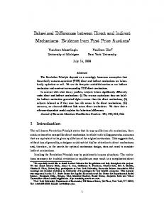
2. Optimal Control Problem: Maximum Range Flight of a Hang Glider The maximum range ight of a hang glider through a given thermal can be modelled by the following optimal control problem: The vehicle is approximately described as a point mass subject to its weight W , a lift force L perpendicular to the velocity vr relative to the air, and a drag force D opposite to vr . The relative velocity vector vr is at an angle  relative to the horizontal plane. The motion of the hang glider is restricted to a vertical plane. Thus we have four state variables: the horizontal distance x , the altitude y , the horizontal absolute velocity component vx , and the vertical absolute velocity component vy ; see Fig. 1. The given thermal is assumed to have a distribution with respect to the horizontal distance x as given by the upward wind velocity ua (x) ,   x

ua (x) = ua max exp ? R ? 2:5

2  

x

1 ? R ? 2:5

2 

(1)

where 5 R denotes the horizontal extent of the thermal (here R = 100 [m] ) and ua max gives the maximal upwind velocity (here ua max = 2:5 [m s?1] ). A

similar problem is described in [25] for the minimum time ight of a sailplane through a thermal of the type (1).

Fig. 1. Forces and velocity components. Thus we have the following equations of motion,

x_ = vx ; y_ = vy ; with



v_ x = m1 (?L sin  ? D cos ) ; v_ y = m1 (L cos  ? D sin  ? W )

(2)



q v ? u ( x ) y a ; vr = vx2 + (vy ? ua (x))2 ;  = arctan vx L = cL 21  S vr2 ; D = cD (cL) 12  S vr2 ; W = m g :

The hang glider is controlled via the lift coecient cL . The drag coecient cD is assumed to be a quadratic function of the lift coecient. Based on data for a high performance hang glider of the type Saphir 17 (see [36]), this leads to the quadratic polar cD (cL ) = cD0 + k c2L (3) with values cD0 = 0:034 and k = 0:069662 . In addition, the lift coecient is constrained, cL  cL max := 1:4 : (4) Further constants are m = 100 [kg] (mass of vehicle and pilot), S = 14 [m2] (wing area),  = 1:13 [kg m?3] (air density corresponding to standard pressure and temperature at a height of about 1000 m above sea level), and g = 9:81 [m s?2] (gravitational acceleration).

The model is completed by the following boundary conditions where the direct starting and landing phase is excluded because of the diculties in modelling them appropriately,

x(0) = 0 [m] ; y(0) = 1000 [m] ; vx (0) = vx McC := 13:23 [m=s] ; vy (0) = vy McC := ?1:288 [m=s] ;

x(tf ) =! max ; y(tf ) = 900 [m] ; vx (tf ) = vx McC [m=s] ; vy (tf ) = vy McC [m=s] :

(5)

A given dierence between initial and terminal altitude is to be used to maximize the range with initial and terminal velocity prescribed. Here, vx McC and vy McC denote the components of the so-called McCready velocity, which is associated with the velocity of best gliding. By means of the minimum principle the optimal control function can be eliminated in terms of the state and the adjoint variables; cf., e.g., [2]. Hence, we have 8 1 > < cfree L := ?

cL = > :

cL max

vx sin  ? vy cos  free 2k vx cos  + vy sin  if cL < cL max if cfree L  cL max

(6)

where the adjoint variables satisfy the dierential equations

_  = ? @H @  ;  2 fx; y; vx; vy g

(7)

with the Hamiltonian de ned by

H = x x_ + y y_ + vx v_ x + vy v_ y :

(8)

To give an impression of the complexity of the adjoint variables, one of the equations is presented here, "



vx2 _ x = m1 vx ?cL  S (vy ? ua (x)) sin  ? L p 2 vx + (vy ? ua (x))23

? cD (cL )  S (vy ? ua (x)) cos  + D p 2vx (vy ? ua (x)) 23 vx + (vy ? ua (x)) 

+ vy cL  S (vy ? ua (x)) cos  ? L p vx (vy ? ua (x)) 3 vx2 + (vy ? ua (x))2



vx2

? cD (cL )  S (vy ? ua (x)) sin  ? D p 

  x


ua (x) + ua max exp ? R ? 2:5

#

vx2 + (vy ? ua (x))23

2   2  x

? R R ? 2:5



:

The boundary-value problem is completed by the transversality conditions

x (tf ) = ?1 ; H jt=tf = 0 :

(9)

After the transformation  := t=tf of the interval [0; tf ] onto [0; 1] , the equations (2), (7), (5), and (9) describe a two-point boundary-value problem for 9 unknowns. Note that the nal time tf then is an additional dependent variable introduced by that transformation. The right-hand side of the system of dierential equations depends via (6) on the sign of a so-called switching function,

S := cfree L ? cL max :

(10)

Thus, we have a so-called two-point boundary-value problem with switching function. Alternatively, we can formulate a multipoint boundary-value problem which is based on a hypothesis of the switching structure. For example, if the optimal trajectory is assumed to have one interior constrained subarc, a multipoint boundaryvalue problem can be stated having one additional interior boundary condition at both the entry and the exit point of that constrained subarc. Because of the continuity of the control function, the interior boundary conditions are

cfree L jt=tentry = cL max jt=tentry ; cfree L jt=texit = cL max jt=texit :

(11)

With respect to the convergence behaviour of the multiple shooting method, the latter formulation is more advantageous than the formulation using switching functions; see [28]. Note that it is, in this case, important to examine the solution of the multipoint boundary-value problem whether the sign of the switching function (10) and the control law according to (6) correspond with the control law based on the hypothesis. See [8, 9] for techniques how to reveal and adapt the switching structure for problems with multiple subarcs. Herewith all information is provided to treat the problem by an indirect method; the above analysis can be omitted when applying a direct method.

3. Numerical Procedure: Combination of Direct and Indirect Methods 3.1 Attempt of the construction of a starting trajectory using multiple shooting. Using the indirect approach, the most promising way to obtain a candidate for an optimal solution of a given problem is to embed this problem into a family of subproblems. By homotopy techniques the solution of one problem out of that family then serves as an initial guess for the solution of a neighboring problem. Starting with a simpli ed problem, the given optimal control problem can be solved via the solution of a whole chain of boundary-value problems.

For the problem under consideration, we rst omit the control constraint (4), and we also neglect the upwind by setting the parameter ua max = 0 . So, the maximum lift coecient cL max as well as ua max will play the role of homotopy parameters. Then we have the following information about the adjoint variables x and y ,

x (t) = const = ?1 ; y (t) = const : However, no information about vx and vy is available. This poor knowledge of the adjoint variables causes the numerical integration to fail for both backward and forward integration unless the adjoint variables are properly guessed. Usually many attempts must be undertaken to obtain a trajectory which at least has some relevancy. This trajectory or may be a part of it then would provide the rst boundary-value problem of the aforementioned family from which we could start the homotopy.

3.2 Construction of a starting trajectory using direct collocation. Apply-

ing the direct collocation method [33], convergence cannot be obtained for the full model directly. We have to apply homotopy techniques, too. For lower initial velocity components, here vx (0) = 11 [m s?1] and vy (0) = ?1:1 [m s?1] , and for the simpli ed model where both the upwind and the constraint of the lift coecient are neglected, a solution can be obtained by the direct collocation method even when starting the iteration with the following simple initial guess. This initial estimate is constituted by the linear polynomial which interpolates the boundary values for the state variables and by cL  1 for the control function. The McCready velocity components and the upwind are then introduced step by step. For the upwind the parameter ua max is increased to ua max = 2 [m s?1] in steps of 0:5 [m s?1] . A grid of 21 equidistant points is used for the discretization of the time interval throughout the whole homotopy. Thereafter, the approximation is improved by a grid re nement; 37 non-equidistant grid points are chosen so that the error function d( ) := maxi i jfi (p; u;  ) ? p0i ( )j with appropriate scaling factors i > 0 is approximately equally distributed over the interval [0; 1] . Here, p denotes the piecewise cubic vector polynomial interpolating the state vector and its derivatives at the grid points. The variable u denotes the control function, and the fi's are the components of the right-hand

side. The variable  := t=tf is the normalized time. We nally end up with an approximate solution provided by the collocation method from which an approximation of the adjoint variables can be obtained according to [34] with an accuracy sucient to yield convergence by the multiple shooting software package [28]. Figures 2{6 show the solution obtained by the direct collocation method (dashed line) and the improved solution obtained by the multiple shooting method (solid line). The dierences for the horizontal distance x and the altitude y are below the drawing accuracy. The approximation for the velocity component vy shows the largest dierences; see Fig. 5. The values for the maximum range are x(tf ) = 1201:65 [m] with tf = 96:444 [s] obtained by the collocation method and x(tf ) = 1201:63 [m] with tf = 96:438 [s] obtained by the multiple shooting method. In Figure 3 the grid points are marked which have been used for the collocation method. Figures 7{9 show the accuracy of the initial guess of the adjoint variables based on their relationship, according to [34], to the multipliers associated with the nonlinear programming problem. Instead of the graph of the constant adjoint variable y , its approximations are given here: we obtain y  ?10:275 from the collocation method and y  ?10:274 from the multiple shooting method. The diculties in obtaining the numerical solution of the problem are caused by the high sensitivity of the solution with respect to its initial values. A numerical integration of the initial-value problem associated with the solution of the boundary-value problem fails if the integration is carried through over the entire

ight time interval at one stroke. However, the numerical integration of the initialvalue problem can be carried through if, as in the multiple shooting algorithm, a series of initial-value problems is solved over smaller subintervals, where the initial values are always rede ned at the grid points of the discretization using the approximation obtained by the multiple shooting method. The dierent pieces of the trajectory then match with an accuracy of at least 5 digits. That sensitivity also explains why such a relatively large number of grid points is to be used when going over from the collocation method to the multiple shooting method. The higher number of grid points provides a better estimate of the adjoint variables. As a rule of thumb, the adjoint variables must be approximated to an accuracy of at least 2 digits to provide convergence of the multiple shooting iteration if the problem to be solved is as sensitive as the hang glider problem. During the subsequent homotopy steps with the multiple shooting method, the number of multiple shooting nodes can then be decreased again. The question now arises when the transition from the collocation to the multiple shooting method should be done. Generally speaking, the transition should be done preferably for a simpler model. For example, the transition fails when the control variable inequality constraint, too, is taken into account for the solution using the collocation method. On the other hand, if the transition is made for a too simple version of the problem as in [27] where the dierence between initial and terminal

Fig. 2. Horizontal distance versus time;

control constraint omitted, maximum upwind of 2 [m s?1] .

Fig. 3. Altitude versus time;

control constraint omitted, maximum upwind of 2 [m s?1] .

Fig. 4. Horizontal velocity component versus time;

control constraint omitted, maximum upwind of 2 [m s?1] .

Fig. 5. Vertical velocity component versus time;

control constraint omitted, maximum upwind of 2 [m s?1] .

Fig. 6. lift coecient versus time;

control constraint omitted, maximum upwind of 2 [m s?1] .

Fig. 7. Adjoint variable x versus time;

control constraint omitted, maximum upwind of 2 [m s?1] .

Fig. 8. Adjoint variable vx versus time;

control constraint omitted, maximum upwind of 2 [m s?1] .

Fig. 9. Adjoint variable vy versus time;

control constraint omitted, maximum upwind of 2 [m s?1] .

altitude is reduced to 10 [m] and where the upwind as well as the constraint of the lift coecient are also neglected at the beginning, a higher amount of computation is needed because of the smaller domain of convergence of the multiple shooting method. This is caused by the smaller homotopy step sizes. Following this way, the step size for the rst homotopy where the dierence between initial and terminal altitude must be increased varies between about 10?3 [m] to about 2 [m] when using the multiple shooting method. In a second homotopy, the eect of the thermal must be then brought into the game by increasing the parameter ua max . Thereby, the minimum homotopy step size is 10?2 [m s?1] . Recall the homotopy step size of 0:5 [m s?1] for ua max when using the direct collocation method.

3.3 Introducing the control variable inequality constraint using homotopy and multiple shooting. From Fig. 6, we easily obtain a hypothesis of the

switching structure: there will be only one constrained subarc when introducing the control constraint via the parameter cL max moderately. Some of the results for this homotopy are given in Figs. 10{12. The solid lines indicate the extremal values cL max = 2:38 (start of the homotopy) and cL max = 1:4 (end of the homotopy); compare Figs. 4 and 5, too. The intermediate values cL max = 2:0 and cL max = 1:7 are given by the dashed and the dashed-dotted lines, respectively.

4. Numerical Results: The Optimal Trajectory To complete the solution, a very last homotopy step must be performed to achieve the desired maximum upwind of ua max = 2:5 m s?1 . Figures 13{17 show the optimal trajectory obtained by the multiple shooting method. The maximum range is x(tf ) = 1247:60 [m] , the nal time is tf = 98:380 [s] , and the switching times are tentry = 23:301 [s] and texit = 33:250 [s] . The two switching points are indicated in the gures by the vertical dashed lines. The results indicate the gain of range caused by the upwind. To increase the potential energy, the altitude has to be increased. To stay as long as possible in the upwind, the horizontal velocity component has to be decreased. Comparing the results for the maximum range trajectory of the hang glider presented here with the minimum time trajectory of a sailplane presented in [25], we see that the twodimensional model still gives meaningful results for upwind velocities considered here. In the sailplane problem of [25] strong upwind velocities cause a breakdown of the vertical plane model. The optimal trajectory there shows a horizontal velocity component which is negative in the upwind and indicates that the pilot should gain altitude by ying circles in the thermal. This point of a model breakdown is, however, not reached here.

Fig. 10. Lift coecient versus normalized time

for decreasing maximum lift coecient.

Fig. 11. Horizontal velocity component versus normalized time for decreasing maximum lift coecient.

Fig. 12. Vertical velocity component versus normalized time for decreasing maximum lift coecient.

Fig. 13. Lift coecient versus normalized time; optimal trajectory.

Fig. 14. Horizontal distance versus normalized time; optimal trajectory.

Fig. 15. Altitude versus normalized time; optimal trajectory.

Fig. 16. Horizontal velocity component versus normalized time; optimal trajectory.

Fig. 17. Vertical velocity component versus normalized time; optimal trajectory.

5. Conclusions Despite the superiority of the multiple shooting method with respect to accuracy and reliability, which is hardly obtainable by any other method for the solution of optimal control problems, its use is often dicult and laborious since an appropriate guess of initial data, in particular, of the adjoint variables as well as of the switching points must be provided. In this paper it is shown how to overcome this obstacle when solving a real-life problem. By using a direct collocation method the adjoint variables can be estimated from the Lagrange parameters of the underlying nonlinear programming problem. For problems of moderate degree of complexity, the approximations of both the state and the adjoint variables provided by the direct collocation method are accurate enough to yield convergence with the multiple shooting method. At this point of investigation homotopy techniques still must be used to introduce inequality constraints imposed on the model. Future investigations will try to ll this gap to obtain also inequality-constrained optimal solutions by multiple shooting directly using a pre-computation with an improved direct collocation method.

Acknowledgements This research was supported by the German National Science Foundation (Deutsche Forschungsgemeinschaft) through the Sonderforschungsbereich 255 (Transatmospharische Flugsysteme)

References

[1] Bock, H. G. and Plitt, K. J.: A Multiple Shooting Algorithm for Direct Solution of Optimal Control Problems, Proceedings of the 9th IFAC Worldcongress, Budapest, 1984, Vol. IX, Colloquia 14.2, 09.2, 1984. [2] Bryson, A. E. and Ho, Y. C.: Applied Optimal Control, New York: Hemisphere (Rev. Printing), 1975. [3] Bulirsch, R.: Die Mehrzielmethode zur numerischen Losung von nichtlinearen Randwertproblemen und Aufgaben der optimalen Steuerung, Carl-Cranz Gesellschaft, Oberpfaenhofen, Report der Carl-Cranz Gesellschaft, 1971; Munich University of Technology, Department of Mathematics, Munich, Reprint, 1985. [4] Bulirsch, R. and Callies, R.: Optimal Trajectories for an Ion Driven Spacecraft from Earth to the Planetoid Vesta, Proc. of the AIAA Guidance, Navigation and Control Conference, New Orleans, 1991, AIAA Paper No. 91-2683, 1991. [5] Bulirsch, R. and Callies, R.: Optimal Trajectories for a Multiple Rendezvous Mission to Asteroids, 42nd International Astronautical Congress, Montreal, 1991, IAF-Paper No. IAF-91-342, 1991. [6] Bulirsch, R., Chudej, K., and Reinsch, K. D.: Optimal Ascent and Staging of a Two-Stage Space Vehicle System, Jahrestagung der Deutschen Gesellschaft fur Luftund Raumfahrt, Friedrichshafen, 1990, DGLR-Jahrbuch 1990, Vol. 1, 243{249, 1990.

[7] Bulirsch, R. and Chudej, K.: Ascent Optimization of an Airbreathing Space Vehicle, Proc. of the AIAA Guidance, Navigation and Control Conference, New Orleans, 1991, AIAA Paper No. 91-2656, 1991. [8] Bulirsch, R., Montrone, F., and Pesch, H. J.: Abort Landing in the Presence of a Windshear as a Minimax Optimal Control Problem, Part 1: Necessary Conditions, J. of Optimization Theory and Applications 70, 1{23, 1991. [9] Bulirsch, R., Montrone, F., and Pesch, H. J.: Abort Landing in the Presence of a Windshear as a Minimax Optimal Control Problem, Part 2: Multiple Shooting and Homotopy, J. of Optimization Theory and Applications 70, 221{252, 1991. [10] Callies, R.: Optimal Design of a Mission to Neptune, in: Bulirsch, R., Miele, A., Stoer, J., and Well, K. H. (eds): Optimal Control, Proc. of the Conf. in Optimal Control and Variational Calculus, Oberwolfach, 1991, Lecture Notes in Control and Information Sciences, Berlin, Heidelberg, New York, London, Paris, Tokyo: Springer, this issue. [11] Chernousko, F. L. and Lyubushin, A. A.: Method of Successive Approximation for Solution of Optimal Control Problems, Optimal Control Applications and Methods 3, 101{114, 1982. [12] Deu hard, P.: A Relaxation Strategy for the Modi ed Newton Method, in: Bulirsch, R., Oettli, W., and Stoer, J. (eds.), Optimization and Optimal Control, Proceedings of a Conference Held at Oberwolfach, 1974, Lecture Notes in Mathematics 477, Berlin, Heidelberg, New York: Springer, 59{73, 1975. [13] Deu hard, P.: A Modi ed Newton Method for the Solution of Ill-conditioned Systems of Nonlinear Equations with Application to Multiple Shooting, Numerische Mathematik 22, 289{315, 1974. [14] Deu hard, P. and Bader, G.: Multiple Shooting Techniques Revisited, in: Deu hard, P. and Hairer, E. (eds.), Numerical Treatment of Inverse Problems in Dierential and Integral Equations, Proceedings of an International Workshop, Heidelberg, 1982, Progress in Scienti c Computing 2, Boston: Birkhauser, 74{94, 1983. [15] Gottlieb, R. G.: Rapid Convergence to Optimum Solutions Using a Min-H Strategy, AIAA J. 5, 322{329, 1967. [16] Hargraves, C. R. and Paris, S. W.: Direct Trajectory Optimization Using Nonlinear Programming and Collocation, AIAA Journal of Guidance and Control 10, 338{342, 1987. [17] Hiltmann, P.: Numerische Losung von Mehrpunkt-Randwertproblemen und Aufgaben der optimalen Steuerung mit Steuerfunktionen uber endlichdimensionalen Raumen, Munich University of Technology, Department of Mathematics, Doctoral Thesis, 1990. [18] Horn, K.: Solution of the Optimal Control Problem Using the Software Package STOMP, to appear in: Bernhard, P. and Bourdache-Siguerdidjane, H. (eds.), Proc. of the 8th IFAC Workshop on Control Applications of Nonlinear Programming and Optimization, Paris, 1989, Oxford: IFAC Publications, 1991. [19] Jansch, C. and Paus, M.: Aircraft Trajectory Optimization with Direct Collocation Using Movable Gridpoints, in: Proceedings of the American Control Conference, San Diego, 262{267, 1990.

[20] Jansch, C., Schnepper, K., and Well, K. H.: Ascent and Descent Trajectory Optimization of Ariane V/Hermes, in: AGARD Conf. Proc. No. 489 on Space Vehicle Flight Mechanics, 75th Symp. of the AGARD Flight Mechanics Panel, Luxembourg, 1989. [21] Kiehl, M: Vectorizing the Multiple-Shooting Method for the Solution of BoundaryValue Problems and Optimal-Control Problems, in: Dongarra, J., Du, I., Ganey, P., and McKee, S. (eds.), Proceedings of the 2nd International Conference on Vector and Parallel Computing Issues in Applied Research and Development, Troms, 1988, London: Ellis Horwood, 179{188, 1989. [22] Kelley, H. J., Kopp, R. E., and Moyer, H. G.: Successive Approximation Techniques for Trajectory Optimization, Proc. Symp. on Vehicle System Optimization, New York, 1961. [23] Kraft, D.: FORTRAN Computer Programs for Solving Optimal Control Problems, Deutsche Forschungs- und Versuchsanstalt fur Luft- und Raumfahrt, Oberpfaenhofen, Report 80-03, 1980. [24] Kraft, D.: On Converting Optimal Control Problems into Nonlinear Programming Codes, in: Schittkowski, K. (ed.) Computational Mathematical Programming, Berlin: Springer (NATO ASI Series 15), 261{280, 1985. [25] Lorenz, J.: Numerical Solution of the Minimum-Time Flight of a Glider Through a Thermal by Use of Multiple Shooting Methods, Optimal Control Applications and Methods 6, 125{140, 1985. [26] Miele, A.: Gradient Algorithms for the Optimization of Dynamic Systems, in: Leondes, C. T., Control and Dynamic Systems 16, New York: Academic Press, 1{52, 1980. [27] Nerz, E.: Optimale Steuerung eines Hangegleiters, Munich University of Technology, Department of Mathematics, Diploma Thesis, 1990. [28] Oberle, H. J.: Numerische Berechnung optimaler Steuerungen von Heizung und Kuhlung fur ein realistisches Sonnenhausmodell, Habilitationsschrift, Munich University of Technology, Munich, Germany, 1982. [29] Oberle, H. J.: Numerical Computation of Singular Control Functions for a TwoLink Robot Arm, in: Bulirsch, R., Miele, A., Stoer, J., and Well, K. H. (eds): Optimal Control, Proc. of the Conf. in Optimal Control and Variational Calculus, Oberwolfach, 1986, Lecture Notes in Control and Information Sciences 95, Berlin, Heidelberg, New York, London, Paris, Tokyo: Springer, 244{253, 1987. [30] Oberle, H. J.: Numerical Computation of Singular Functions in Trajectory Optimization Problems, J. Guidance and Control 13, 153{159, 1990. [31] Renes, J. J.: On the Use of Splines and Collocation in a Trajectory Optimization Algorithm Based on Mathematical Programming, National Aerospace Laboratory, Amsterdam, Report No. NLR-TR-78016 U, 1978. [32] Stoer, J. and Bulirsch, R.: Introduction to Numerical Analysis, New York: Springer, 1980. [33] von Stryk, O.: Numerical Solution of Optimal Control Problems by Direct Collocation, in: Bulirsch, R., Miele, A., Stoer, J., and Well, K. H. (eds): Optimal Control, Proc. of the Conf. in Optimal Control and Variational Calculus, Oberwolfach, 1991,

Lecture Notes in Control and Information Sciences, Berlin, Heidelberg, New York, London, Paris, Tokyo: Springer, this issue. [34] von Stryk, O. and Bulirsch, R.: Direct and Indirect Methods for Trajectory Optimization, Annals of Operations Research 37, 357{373, 1992. [35] Tolle, H.: Optimierungsverfahren, Berlin: Springer, 1971. [36] Drachen iegermagazin, Munchen: Ringier Verlag, issue 7, 1988.

Prof. Dr. Roland Bulirsch, Dipl. Math. Edda Nerz, Priv.-Doz. Dr. Hans Josef Pesch, Dipl. Math. Oskar von Stryk, Mathematisches Institut, Technische Universitat Munchen, Postfach 20 24 20, D{8000 Munchen 2