Mar 3, 2000 - We call graph drawing problems in which subsets of vertices and edges need to be labeled ... Download to read the full conference paper text.
Combining Graph Labeling and Compaction? (Extended Abstract) Gunnar W. Klau and Petra Mutzel Max–Planck–Institut f¨ ur Informatik Im Stadtwald, D–66123 Saarbr¨ ucken, Germany {guwek,mutzel}@mpi-sb.mpg.de
Abstract. Combinations of graph drawing and map labeling problems yield challenging mathematical problems and have direct applications, e.g., in automation engineering. We call graph drawing problems in which subsets of vertices and edges need to be labeled graph labeling problems. Unlike in map labeling where the position of the objects is specified in the input, the coordinates of vertices and edges in a graph labeling problem instance have yet to be determined and thus create additional degrees of freedom. We concentrate on the Compaction and Labeling (COLA) Problem: Given an orthogonal representation—as produced by algorithms within the topology–shape–metrics paradigm—and some label information, the task is to generate a labeled orthogonal embedding with minimum total edge length. We characterize feasible solutions of the COLA problem extending an existing framework for solving pure compaction problems. Based on the graph–theoretical characterization, we present a branch–and–cut algorithm which computes optimally labeled orthogonal drawings for given instances of the COLA problem. First computational experiments on a benchmark set of practical instances show that our method is superior to the traditional approach of applying map labeling algorithms to graph drawings. To our knowledge, this is the first algorithm especially designed to solve graph labeling problems.
1
Introduction
The area of graph drawing provides an ample variety of algorithms that produce aesthetically pleasing layouts of graphs [DETT99]. At the same time, there are sophisticated techniques to generate provably good labelings of cartographic maps [WS]. Combinations of problems from both areas yield challenging mathematical problems and have direct applications, e.g., the automatic layout of state diagrams in automation engineering or the drawing of schematic maps such as subway maps. Unlike in map labeling where the position of the objects is specified in the input, the coordinates of vertices and edges in a graph drawing problem instance have yet to be determined and thus create additional degrees of freedom. ?
This work is partially supported by the Bundesministerium f¨ ur Bildung, Wissenschaft, Forschung und Technologie (No. 03–MU7MP1–4).
J. Kratochv´ıl (Ed.): GD’99, LNCS 1731, pp. 27–37, 1999. c Springer-Verlag Berlin Heidelberg 1999
28
G.W. Klau and P. Mutzel
We call the class of graph drawing problems where subsets of vertices and edges have to be labeled graph labeling problems. So far, problems from this class have only been attacked by applying map labeling algorithms to graph drawings [KT97,IL97]. Figure 1 shows a labeled drawing for a state diagram; first the underlying graph has been drawn, in a last step the labels have been placed with an optimal labeling strategy. This forces some labels to either overlap parts of the drawing or to be placed far away from the vertices to which they should be attached. Another approach could be to model each label as a vertex of fixed size and then apply a graph drawing algorithm which can cope with vertices of different sizes. This treatment increases the vertex degrees and may destroy existing structural properties in the graph—for the drawing of state diagrams this leads to a loss of orthogonality and unacceptable area consumption.
Fig. 1. A state diagram; first drawn then labeled
In this paper we concentrate on a special graph labeling problem: the Compaction and Labeling (COLA) Problem. Graph drawing algorithms in the topology–shape–metrics paradigm [DETT99] produce in an intermediate step a so– called orthogonal representation H, i.e., an extended planar representation. In addition to the topological information, H contains for each edge information about the order of bends and the angle formed with the following edge in the appropriate face. In the compaction phase of the paradigm, the goal is to minimize the area or the total edge length of the resulting orthogonal drawing. The COLA problem unifies the problem to find a drawing respecting the given shape and an additional labeling task: A set of labels, each of which is fixed in size, is assigned to every vertex v. Each of the labels must be placed so that it touches v in at
Combining Graph Labeling and Compaction
29
least one point and does not overlap other objects. We are given a set of k labels L = {λ1 , λ2 , . . . , λk }, two functions w : L → Q, h : L → Q determining the width and height of each label, and a third function a : L → V denoting the vertex a(λ) to which the label λ should be attached. We are looking for a labeled orthogonal embedding with short edges in which each label is placed correctly, and no labels overlap the drawing. In this paper we give a characterization of feasible solutions for the COLA problem. We extend an existing framework for two–dimensional compaction problems in graph drawing [KM99]. Based on the graph–theoretical characterization, we present a first branch–and–cut based algorithm prototype which computes optimally labeled orthogonal drawings for given instances of the COLA problem. To our knowledge, this is the first algorithm especially designed to solve graph labeling problems. Section 2 introduces the graph–theoretical framework. We give a formal definition of the COLA problem in Sect. 3 and show how to integrate the additional labeling problem into the framework. In Sect. 4 we extend an optimal branch– and–cut algorithm so that it solves the COLA problem to optimality and give some first computational results. Finally, we conclude with Sect. 5. Due to space limitations we can only give sketches of the proofs.
2
Constraint Graphs
In this section we introduce the graph–theoretical framework we have developed to solve the COLA problem. An algorithm within the topology–shape–metrics approach [DETT99] produces at the end of the second phase an orthogonal representation H which contains the information about the topology and the shape of the drawing. We call H simple if its number of bends is zero. Every orthogonal representation can be transformed into a simple one by just replacing each bend with an artificial vertex. In order to compute a drawing for H, we must assign coordinates to the vertices and bends. In this paper, we concentrate on pure orthogonal embeddings, but our ideas can be adapted to other drawing standards such as Kandinsky–like embeddings (introduced in [FK96]) or orthogonal box embeddings (subclasses are the big node model from [FK97] and the TSS model from [BMT97], a related class is the quasi–orthogonal model from [KM98]). Pure orthogonal embeddings are only admissible for 4–planar graphs. Each vertex and bend is mapped to a point and edge segments are mapped to horizontal or vertical non–crossing line segments of some minimum length connecting the images of their endpoints. A special case are pure orthogonal grid embeddings as defined in [Tam87]: Here, vertices and bends have integer coordinates. As with representations, we call orthogonal embeddings simple if they do not contain bends. We first focus on the following subproblem of the COLA problem: Given an orthogonal representation H, produce an orthogonal embedding Γ for H
30
G.W. Klau and P. Mutzel
which is—among all such drawings—of minimum total edge length. Recently, Patrignani proved the NP–hardness of this problem [Pat99]. Initial observation leads to the following notion: Incident edges of same direction can be combined, forming the objects to compact. Let Γ be a simple orthogonal drawing of a graph. It induces a partition of the set of edges E into the horizontal set Eh and the vertical set Ev . A horizontal (resp. vertical) subsegment in Γ is a connected component in (V, Eh ) (resp. (V, Ev )). If the component is maximally connected it is also referred to as a segment. The following observations are crucial (see also Fig. 2). – Each edge is a subsegment. – Each vertex v belongs to one unique horizontal and one unique vertical segment, denoted by hor(v) and vert(v). – The limits of a subsegment s are given as follows: Let vl , vr , vb , and vt be the leftmost, rightmost, bottommost, and topmost vertices on s. Then l(s) = vert(vl ), r(s) = vert(vr ), b(s) = hor(vb ), and t(s) = hor(vt ).
v3 v2 v1
s3 s2 s4 s1
v4 s5 v5
Sh = fs1; s2 ; s3 g
Sv = fs4 ; s5 g
i V (si ) E (si ) l(si ) r(si ) b(si ) t(si ) 1 fv1 g fg s4 s4 s1 s1 2 fv2 ; v5 g f(v2 ; v5 )g s4 s5 s2 s2 3 fv3 ; v4 g f(v3 ; v4 )g s4 s5 s3 s3 4 fv1 ; v2 ; v3 g f(v1 ; v2 ); (v2 ; v3 )g s4 s4 s1 s3 5 fv4 ; v5 g f(v4 ; v5 )g s5 s5 s2 s3
Fig. 2. Segments of a simple orthogonal grid drawing and its limits
We provide a necessary and sufficient condition for all feasible solutions of a given instance of the compaction problem. This condition is based on existing paths in the so–called constraint graphs. This pair of directed graphs is similar to the layout graphs known from one–dimensional compaction strategies in VLSI design [Len90]. Nodes in these graphs represent the segments; their weighted arcs characterize relative positioning relations between the segments. We denote by ci the coordinate of segment si . A weight ωij ∈ Q for an arc (si , sj ) indicates that the coordinate difference cj − ci must be at least ωij . Figure 3 shows an example for a pair of constraint graphs. The arcs specify exactly the relative relationships known from the shape of the graph: We call such special pairs of constraint graphs h(Sv , Ah ), (Sh , Av )i shape graphs or a shape description. Note that each horizontal edge in the original graph defines a relative positioning constraint between two vertical segments. Similarly, vertical edges determine constraints between horizontal segments. The characterization of feasible solutions for the two-dimensional compaction problem is based on the following three observations:
Combining Graph Labeling and Compaction
s4
1
s6
1
s5
1
1 s2
s7
31
1
1 s8 s3
1 1
1
s9
1
1 s1
Fig. 3. An orthogonal grid embedding (dotted) and a pair of constraint graphs
1. The arcs of the shape graphs are contained in every pair of constraint graphs corresponding to a drawing reflecting the given shape. 2. Generally, the information in the shape graphs is not sufficient to produce an orthogonal embedding. If this is the case, however, we call such a pair of constraint graphs complete. 3. There are in general many possibilities for extending the shape graphs to a complete pair of constraint graphs. +
We denote by si −→ sj a path of non–negative weight between si and sj . The following is a precise characterization for complete pairs of constraint graphs in terms of paths that must be contained in the arc sets: A pair of graphs is complete if and only if both arc sets do not contain non–negative cycles and for every pair of segments (si , sj ) ∈ S × S one of the following four conditions holds: +
1. r(si ) −→ l(sj ) +
2. r(sj ) −→ l(si )
+
3. t(sj ) −→ b(si )
(1)
+
4. t(si ) −→ b(sj )
If one of the non–negative paths in (1) exists we also call the pair of segments (si , sj ) separated. Note that this definition generalizes the notion of completeness as introduced for the pure compaction problem in [KM99]. There, we have the special case that ωij = 1 for all (si , sj ). We can now express a one–to–one correspondence between these complete extensions and orthogonal embeddings. On the basis of the following theorem, the two–dimensional compaction task can be seen as the search for a complete extension of the given shape graphs leading to minimum total edge length. Theorem 1 ([KM99]). For each simple orthogonal embedding with shape description σ = h(Sv , Ah ), (Sh , Av )i there exists a complete extension τ = h(Sv , Bh ), (Sh , Bv )i of σ and vice versa: Every complete extension τ = h(Sv , Bh ),
32
G.W. Klau and P. Mutzel
(Sh , Bv )i of a shape description σ = h(Sv , Ah ), (Sh , Av )i corresponds to a simple orthogonal embedding with shape description σ.
3
Modeling the Labels
In this section we extend the graph–theoretical formulation of the pure two– dimensional compaction problem so that a feasible solution corresponds to a labeled orthogonal embedding and thus to a solution of the COLA problem. We define the characteristics of a solution for the COLA problem in order to state the COLA problem formally. Definition 1. A labeled orthogonal embedding ΓL for an orthogonal representation H of a planar graph G = (V, E) and a label set L with functions w, h : L → Q and a : L → V fulfills the following properties: 1. ΓL is an orthogonal embedding for H. 2. A label λ ∈ L has size w(λ) × h(λ) and its image intersects with the image of vertex a(λ) at at least one point. 3. A label λ ∈ L does neither overlap nor include other objects. Definition 2. Compaction and Labeling (COLA) problem. Given an orthogonal representation H for a planar graph G = (V, E), a label set L with functions w, h : L → Q, and a : L → V , find a labeled orthogonal embedding for H with minimum total edge length. We model each label λ as a rectangle bounded by the segments lλ , rλ , tλ , and bλ as in Fig. 4. Its limits are linked by two arcs (lλ , rλ ) ∈ Ah and (bλ , tλ ) ∈ Av of weight w(λ) and h(λ), respectively. Unlike the arcs from the previous section, the minimum distance requirements for this type of arcs are determined by the width and height of the corresponding label. Observe that we use the same sort of segments we have introduced in the previous section for the solution of the compaction problem. At this point we introduce a set O containing the objects to compact. It consists of the segments corresponding to consecutive edges of same direction and all the labels. This gives us an important property free of charge: If we can ensure that—as in Sect. 2—all pairs of distinct objects in O are separated, the labels will neither overlap nor will they be crossed by edges of the graph. We will achieve this by giving a more general definition of completeness. We additionally have to guarantee that each label is drawn in the neighborhood of the vertex to which it belongs. Figure 5 shows the possibilities we want to capture with our formulation. According to Def. 1 a label can be placed anywhere close to a vertex, i.e., it must touch the vertex at at least one point. The relative positioning of label λ to its vertex v = a(λ) can be equivalently expressed by the following four conditions: 1. The left side of λ must not lie to the right side of v. 2. The right side of λ must not lie to the left side of v.
Combining Graph Labeling and Compaction
33
t�
t� l�
�
�
l� lv
r�
tv
v
b�
r�
rv
bv
b� Fig. 5. Possibilities for placing a label λ in the neighborhood of a(λ)
Fig. 4. Four segments model a label
3. The bottom side of λ must not lie above the top side of v. 4. The top side of λ must not lie below the bottom side of v. In our graph–theoretical framework this translates into four special arcs of zero weight that have to be included in the pair of constraint graphs (see Fig. 5). For a label λ with a(λ) = v these are (lλ , rv ), (lv , rλ ), (bλ , tv ), and (bv , tλ ), linking the limits of the label to the limits of the vertex. Note that we model vertices whose images are boxes of non–zero size in a similar way as the labels by including them in O and linking them appropriately to the segments that correspond to incident edges. Having introduced these new types of arcs, we can extend the notion of shape description as defined in Sect. 2 to integrate the labels in the framework. Definition 3. A labeled shape description σL of an orthogonal representation H with label information L, w, h, and a is a tuple h(Sv ∪ SLv , Ah ∪ ALh ), (Sh ∪ SLh , Av ∪ ALv )i where h(Sv , Ah ), (Sh , Av )i is a shape description for H and [ [ {lλ , rλ }, ALh = {(lλ , rλ ), (lλ , ra(λ) ), (la(λ) , rλ )}, SLv = λ∈L
SLh =
[
{bλ , tλ },
λ∈L
λ∈L
ALv =
[
{(bλ , tλ ), (bλ , ta(λ) ), (ba(λ) , tλ )} .
λ∈L
Clearly, each instance of the COLA problem uniquely determines a labeled shape description. We can now give a more general formulation of completeness by considering all objects in the set O: A pair of labeled constraint graphs is complete if and only if it does not contain a non–negative cycle and each distinct pair of objects is separated. This generalization leads to the following main result. Theorem 2. For each simple labeled orthogonal embedding with shape description σ = h(Sv , Ah ), (Sh , Av )i and label information L, w, h, a there exists a complete labeled extension τ = h(Sv ∪ SLv , Ah ∪ ALh ), (Sh ∪ SLh , Av ∪ ALh )i of σ and vice versa: Every complete labeled extension τ = h(Sv ∪ SLv , Bh ∪ ALh ), (Sh ∪ SLh , Bv ∪ ALh )i of a labeled shape description σ = h(Sv ∪ SLv , Ah ∪ ALh ), (Sh ∪ SLh , Av ∪ ALh )i corresponds to a simple labeled orthogonal embedding with shape description σ.
34
G.W. Klau and P. Mutzel
Proof (Sketch). The proof is similar to the one in [KM99, Theorem 1], so we give only a sketch of it: For the forward direction, we construct a complete extension of the given labeled shape description σ by inserting the missing information according to the visibility properties in the drawing. Clearly, this excludes non–negative cycles. The separation properties are also fulfilled for all segments because otherwise there would be overlapping objects in the drawing, which is not the case. For the other direction, we give a constructive proof of how to build a labeled orthogonal embedding with a given complete extension of a labeled shape description: As in the proof for the pure compaction setting, we make use of a length assignment to assign the coordinates to the segments—and thus to the vertices, bends, and labels. Again, we are able to show that the resulting drawing is a labeled orthogonal embedding reflecting the shape of H and the labeling information given in L, w, h, and a.
4
Optimal Graph Labeling
In this section we introduce our the ILP formulation to solve the COLA problem to optimality and present first computational results. One way to characterize the set of complete extensions is by means of an integer linear program. We introduce a binary variable xij for each arc (si , sj ) that might be in some extension of the given labeled shape description σL = h(Sv , Ah ), (Sh , Av )i. If (si , sj ) is contained in the extension, the corresponding variable xij is one, otherwise zero. We refer by X to the set of binary variables. Additionally, there is a variable cs ∈ Q for each segment s ∈ S denoting the coordinate of s. The ILP then reads as follows: min
X e∈Eh
cr(e) − cl(e) +
X
ct(e) − cb(e) subject to
(2)
e∈Ev
xro ,lp + xrp ,lo + xto ,bp + xtp ,bo ≥ 1 cj − ci ≥ ωij cj − ci − (M + ωij )xij ≥ −M xij ∈ {0, 1}
∀(o, p) ∈ O × O, o 6= p ∀(si , sj ) ∈ Ah ∪ Av ∀xij ∈ X ∀xij ∈ X
(2.1) (2.2) (2.3) (2.4)
Inequalities (2.1) model the characterization of separation, i.e., the existence of necessary paths between distinct objects in an extension. Inequalities (2.2) force the coordinates to obey the distance rules coded by the weighted arcs in the underlying labeled shape description; the value ωij denotes the minimum distance between si and sj . The same must hold true for the potential additional arcs: Whenever a variable xij is one, we want an inequality of type (2.2), otherwise there should be no restriction on the coordinate variables. This situation is modeled by inequalities (2.3) with the help of a big constant M . We have shown in [KM99] that inequalities (2.2) and (2.3) ensure the absence of non–negative cycles in the extension.
Combining Graph Labeling and Compaction
35
Note that we do not introduce additional decision variables to integrate the labeling task; the choice of where to place a label is performed by the separation properties. A label can be placed wherever it does not interfere with other objects as long as it stays in the neighborhood of the vertex to which it belongs. Moreover, we do not restrict the label placement to a finite number of prescribed places. Of course, the number of possibly non–separated segments is much higher than in an instance of a pure compaction problem. Like the one–to–one correspondence between complete extensions and orthogonal embeddings there is a one–to–one correspondence between feasible solutions of the ILP and complete extensions of the given labeled shape graphs: Theorem 3. For each feasible solution (x, c) of the ILP for a given labeled shape description σL there is a labeled orthogonal embedding with appropriate shape and label information and vice versa. Proof (Sketch). A solution of the ILP corresponds to a complete extension of the labeled shape description σ with appropriate length assignment. The forward direction follows with Theorem 1. Conversely, we can use the information of a labeled embedding to construct a feasible solution of the ILP. We can show that none of the inequalities is violated and that the value of the objective function equals the total edge length. We have extended the existing branch–and–cut framework for the pure compaction problem to solve instances of the COLA problem and have developed a prototype of an optimal compaction and labeling algorithm. We have tested the algorithm with real–world instances from the area of automation engineering and our first computational experiments indicate that we are able to draw and label the state diagrams within moderate computation time. Figure 6 shows the output of the optimal algorithm for the example of Fig. 1. It took the algorithm prototype 29 seconds to compute the optimal solution.
5
Conclusions and Future Plans
We have introduced a combined compaction and labeling problem arising from a practical application in automation engineering. The task is to simultaneously assign consistent edge lengths for a given orthogonal representation which determines the shape of the drawing and to label subsets of vertices. The resulting drawing should have small total edge length and all labels should be placed at the corresponding vertices so that they do not overlap other objects. Already the pure compaction task is NP–hard. We have integrated the labeling problem into an existing graph–theoretical framework for solving two–dimensional compaction problems and have introduced the notion of labeled orthogonal embedding. Inside this framework, we have devised a branch–and–cut algorithm that produces optimal solutions for the COLA problem. Note that we do not require a label to be placed on a finite
36
G.W. Klau and P. Mutzel
�21 �16
�15
�20 �17
�19
�14
�18 �12
�9
�7
�8 �10 �6 �13
�1
�2
�11
�5 �3
�4
Fig. 6. The example from Fig. 1, drawn with the optimal algorithm
set of prescribed places but allow for a continuous movement of the label around the vertex to which it is attached. In the near future, we will provide the implementation of the branch–and– cut algorithm as a module inside the AGD library [AGD99]. We will extensively test the optimal algorithm on real world and randomly generated instances. We will try to develop heuristics in order to apply them at each node in the branch–and–cut tree and want to investigate a possible extension to edge labeling problems. Furthermore, we plan to extend our framework so that it can accomplish some postprocessing tasks like improving the number of bends or crossings and decreasing the sizes of vertices.
References AGD99.
AGD. AGD User Manual. Max-Planck-Institut Saarbr¨ ucken, Universit¨ at Halle, Universit¨ at K¨ oln, 1999. http://www.mpi-sb.mpg.de/AGD. BMT97. T. Biedl, B. Madden, and I. Tollis. The three–phase method: A unified approach to orthogonal graph drawing. In G. Di Battista, editor, Graph Drawing (Proc. GD ’97), volume 1353 of Lecture Notes in Computer Science, pages 391–402. Springer-Verlag, 1997. DETT99. G. Di Battista, P. Eades, R. Tamassia, and I. G. Tollis. Graph Drawing. Prentice Hall, 1999. FK96. U. F¨ oßmeier and M. Kaufmann. Drawing high degree graphs with low bend numbers. In F. J. Brandenburg, editor, Graph Drawing (Proc. GD ’95), volume 1027 of Lecture Notes in Computer Science, pages 254–266. Springer-Verlag, 1996.
Combining Graph Labeling and Compaction FK97.
IL97. KM98. KM99.
KT97. Len90. Pat99. Tam87. WS.
37
U. F¨ oßmeier and M. Kaufmann. Algorithms and area bounds for nonplanar orthogonal drawings. In G. Di Battista, editor, Graph Drawing (Proc. GD ’97), volume 1353 of Lecture Notes in Computer Science, pages 134–145. Springer-Verlag, 1997. C. Iturriaga and A. Lubiw. Elastic labels: The two–axis case. In G. Di Battista, editor, Graph Drawing (Proc. GD ’97), volume 1353 of Lecture Notes in Computer Science, pages 181–192, 1997. G. W. Klau and P. Mutzel. Quasi–orthogonal drawing of planar graphs. Technical Report MPI–I–98–1–013, Max–Planck–Institut f¨ ur Informatik, Saarbr¨ uu ¨cken, May 1998. G. W. Klau and P. Mutzel. Optimal compaction of orthogonal grid drawings. In G. P. Cornu´ejols, editor, Integer Programming and Combinatorial Optimization (IPCO ’99), number 1610 in Springer Lecture Notes in Computer Science, pages 304–319, 1999. K. G. Kakoulis and I. G. Tollis. An algorithm for labeling edges of hierarchical drawings. In G. Di Battista, editor, Graph Drawing (Proc. GD ’97), volume 1353 of Lecture Notes in Computer Science, pages 169–180, 1997. T. Lengauer. Combinatorial Algorithms for Integrated Circuit Layout. John Wiley & Sons, New York, 1990. M. Patrignani. On the complexity of orthogonal compaction. Technical Report RT–DIA–39–99, Dipartimento di Informatica e Automazione, Universit` a degli Studi di Roma Tre, January 1999. R. Tamassia. On embedding a graph in the grid with the minimum number of bends. SIAM J. Comput., 16(3):421–444, 1987. A. Wolff and T. Strijk. The map labeling bibliography. http://www.inf.fu-berlin.de/map-labeling/bibliography.