Stephen F. Smith2. Computer Science Department1 and ..... Lin Xu, Frank Hutter, Holger H. Hoos, and Kevin Leyton-Brown. SATzilla2007: a new & improved ...
Combining Multiple Constraint Solvers: Results on the CPAI’06 Competition Data Matthew Streeter1
Daniel Golovin1
Stephen F. Smith2
Computer Science Department1 and The Robotics Institute2 Carnegie Mellon University Pittsburgh, PA 15213 {matts,dgolovin,sfs}@cs.cmu.edu
Abstract. In a recent paper [5], we presented an algorithm that constructs a schedule for interleaving the execution of two or more solvers, with the goal of obtaining improved average-case running time relative to the fastest individual solver. In this paper, we evaluate this algorithm experimentally using data from the CPAI’06 constraint solver competition.
1
Introduction
Many computational problems that arise in practice are NP-hard and thus are unlikely to admit algorithms with provably good worst-case performance. These problems must nevertheless be solved, and in many problem domains heuristics have been developed that perform much better in practice than a worst-case analysis would guarantee. Unfortunately, the behavior of a heuristic on a previously unseen problem instance can be difficult to predict in advance, and the running times of two different heuristics on the same instance can easily differ by orders of magnitude. For this reason, if a heuristic has been running unsuccessfully for some time it may be worthwhile to suspend the execution of that heuristic and start running a different heuristic instead. Table 1. Behavior of two solvers on three instances from the CPAI’06 competition. Instance
BPrologCSPSolver70a CPU (s)
Abscon 109 ESAC CPU (s)
allIntervalSeries/series-10 fisher/FISCHER1-1-fair pseudoSeries/aim/aim-100-1-6-1
0.021 0.046 ≥ 1800
0.72 ≥ 1800 1.089
The potential reduction in average-case running time that can be achieved by interleaving the execution of multiple heuristics is illustrated in Table 1. Here, although both solvers take > 600 seconds on average, a schedule that simply ran the two solvers in parallel would take less than one second on average.
In this paper, we seek to improve the average-case performance of constraint solvers by interleaving the execution of multiple (currently available) constraint solvers according to a task-switching schedule. We construct taskswitching schedules using a recently-developed algorithm [5] and evaluate their performance using data from the CPAI’06 competition. 1.1
Task-switching schedules
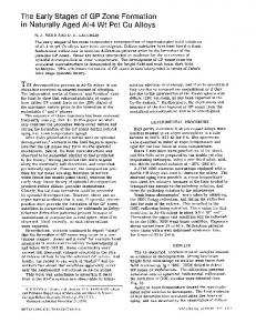
Let H = {h1 , h2 , . . . , hk } be a set of deterministic heuristics, and let X = {x1 , x2 , . . . , xn } be a set of instances of some decision problem. Heuristic hj , when run on instance xi , runs for τi,j time units before returning a (provably correct) “yes” or “no” answer. A task-switching schedule S : Z+ → H specifies, for each integer t ≥ 0, the heuristic S(t) to run from time t to time t + 1. For example, to execute the task-switching schedule depicted in Figure 1 we would run h1 for two time units; then run h2 for two time units, then run h1 for four additional time units, and so on. multi-run
single-run
h1
...
h2 0
2
4
6
8
time Fig. 1. A task-switching schedule.
A task-switching schedule may either be executed in single-run mode or in multi-run mode. The two modes differ in what happens to the heuristic (call it h) that is currently running when the task-switching schedule starts running a new heuristic h0 : in single-run mode, the current run of h is discarded, while in multi-run mode the execution state of h is saved and will be restored if h is run again. For any schedule S, let csi (S) denote the time S takes to solve xi when S is executed in single-run mode and let cm i (S) denote the time it takes when executed in multi-run mode.1 For example, if heuristics h1 and h2 both require 3 time units to solve instance xi (i.e., τi,1 = τi,2 = 3), the task-switching schedule S depicted in Figure 1 will require 5 time units to solve x if it is executed in multi-run mode but will require 7 time units if it is executed in single-run mode s (i.e., cm i (S) = 5 and ci (S) = 7). We now consider the problem of computing a good task-switching schedule. That is, given as input the matrix τ , we would like to compute a schedule 1
Formally, cm i (S) is the smallest integer t such that for some heuristic hj , |{t0 < t : S(t0 ) = hj }| = τi,j . Similarly, csi (S) is the smallest integer t such that, for some heuristic hj , S(t − τi,j ) = S(t − τi,j + 1) = S(t − τi,j + 2) = . . . = S(t − 1) = hj .
Pn Pn that minimizes i=1 csi (S) (or i=1 cm i (S)). Of course, we would not use the resulting task-switching schedule to solve instances in X (which we must already have solved in order to fill in the table τ ). Rather, we would hope that a taskswitching schedule that performs well on the instances in X would also perform well on similar problem instances, which we would be able to solve more quickly via the task-switching schedule. Unfortunately, it is NP-hard to compute even an approximately optimal taskswitching schedule. This follows from the fact that the problem of computing an optimal task-switching schedule generalizes min-sum set cover. Feige et al. [1] showed that it is NP-hard to approximate min-sum set cover within a factor of α for any α < 4, and gave a greedy algorithm that achieves the optimal approximation ratio of 4. In [5], we showed how to generalize this greedy algorithm to obtain a 4-approximation to the optimal task-switching schedule. Our results are summarized in the following theorem. Pn Theorem 1. Let C ∗ = minS i=1 cm api (S). There exists a poly-time Pn greedy m m proximation algorithm that returns a schedule S m such that c (S ) ≤ i=1 i ∗ s 4C . A different greedy approximation algorithm returns a schedule S such that Pn s s ∗ i=1 ci (S ) ≤ 4C . In [5] we also derived bounds on the number of training instances required in order to PAC-learn an optimal (or approximately optimal) schedule for instances drawn independently from a probability distribution. We also developed an online algorithm that receives a sequence hx1 , x2 , . . . , xn i of problem instances one at a time, and solves each instance (via a task-switching schedule) before moving on to the next. 1.2
Related work
Our work is closely related to previous work on algorithm portfolios [2, 3]. An algorithm portfolio consists of a set of heuristics that are run in parallel (or interleaved on a single processor) according to some schedule. The schedules considered in previous work simply run each heuristic in parallel at equal strength and assign each heuristic a fixed restart threshold. The term “algorithm portfolio” has also been used to describe algorithms such as SATzilla [6], which use machine learning to attempt predict which heuristic will solve a given instance the fastest and then run that heuristic exclusively. Task-switching schedules were introduced in a recent paper by Sayag et al. [4], who gave an exact algorithm for computing an optimal task-switching schedule (as already mentioned, doing so is NP-hard, and the running time of their algorithm is exponential in the number of heuristics). For a more detailed discussion of related work, see [5].
2
Results
In this section, we use the greedy algorithms alluded to in Theorem 1 to construct task-switching schedules for interleaving solvers from the CPAI’06 competition.
To do so, we used the data available on the competition web site2 to determine the running time of each constraint solver on each benchmark instance. If a solver did not return a solution within the half hour time limit, we artificially set its running time equal to half an hour. We used this data as input to our greedy approximation algorithms. Note that in performing these experiments, we did not actually run any of the constraint solvers. One might worry that task-switching schedules computed in this way are highly tuned to the specific benchmark instances that were used in the competition. To address this concern, we evaluate our task-switching schedules using leave-one-out cross-validation. The instances in the CPAI’06 competition were divided into five categories: 2-ARY-EXT, 2-ARY-INT, GLOBAL, N-ARY-EXT, and N-ARY-INT. We performed separate experiments on the instances in each category. We present the results for the category N-ARY-INT in detail, then summarize the results for the other four categories. 2.1
Results for category N-ARY-INT
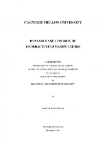
The CPAI’06 competition included 925 instances in the N-ARY-INT category. Of the 14 solvers that were run on these instances, two produced incorrect answers for one or more instances and were excluded from the competition. 726 of the 925 instances were solved by at least one of the 12 remaining solvers within the half hour time limit. We use these 726 instances and these 12 solvers in our experiments. Table 2 displays the number of instances solved within the half hour time limit as well as the average CPU time for each of the 12 solvers as well as four schedules: Greedy m , Greedy s , P arallelm , and P arallels . Greedy m is the schedule S m from Theorem 1 executed in multi-run mode, and similarly Greedy s is the schedule S s from Theorem 1 executed in single-run mode. P arallelm is a schedule that runs all 12 heuristics in parallel, each at equal strength. P arallels is a single-run version of P arallelm which first runs each heuristic for 1 second, then runs each heuristic for 2 seconds, then runs each heuristic for 4 seconds, and so on. As shown in Table 2, the two greedy schedules outperform each of the 12 original solvers as well as the two parallel schedules, both in terms of average CPU time and in terms of the number of instances solved within the half hour time limit. Note that the results listed for the schedules executed in multi-run mode are optimistic in that they assume there is no overhead associated with keeping multiple runs in memory; however there is no such issue with the schedules executed in single-run mode. Also note that because we artificially set a solver’s CPU time equal to the half hour time limit for instances it did not solve, the values for the average CPU time of the 12 heuristics are actually lower bounds, and using the (unknown) actual values could significantly improve our results. Figure 2 illustrates the task-switching schedule Greedy s . 2
http://www.cril.univ-artois.fr/CPAI06/
Table 2. Results for category N-ARY-INT (cross-validation results are parenthesized). Solver
Num. solved Avg. CPU (s)
m
Greedy Greedys Parallelm Parallels BPrologCSPSolver70a Abscon 109 ESAC Abscon 109 AC sugar CSPtoSAT+minisat CSP4J - MAC CSP4J - Combo galac galacJ Tramontane Mistral sat4jCSP
706 (701) 631 (625) 630 614 579 509 490 431 395 370 364 352 331 313 304 228
338 (407) 395 (498) 2460 4896 636 614 659 766 888 963 998 990 1043 1075 1103 1264
BPrologCSPSolver70a Abscon 109 ESAC Abscon 109 AC sugar CSPtoSAT+minisat CSP4J - MAC galac 0.01
0.1
1
10
100
1000
time (s) Fig. 2. The task-switching schedule Greedy s .
To address the possibility of overfitting, we evaluated the task-switching schedules returned by the greedy algorithm using leave-one-out cross-validation.3 The cross-validation results appear in parentheses in Table 2. The number of instances solved by Greedy s decreased by about 1% under cross-validation, while the average CPU time increased by about 26%. The results for Greedy m were similar.
3
Leave-one-out cross-validation is performed as follows: for each instance, we remove that instance from the matrix τ and run the greedy algorithm on the remaining data to obtain a schedule to use in solving that instance.
2.2
Summary of results for all categories
We performed similar experiments on the instances in the four remaining categories: 2-ARY-EXT, 2-ARY-INT, GLOBAL, and N-ARY-EXT. In each experiment, we removed solvers that produced an incorrect answer on one or more instances, and we removed instances that none of the solvers could solve within the half hour time limit. The results for all five instance categories are summarized in Table 3. In four out of five categories, the two greedy schedules outperform the corresponding parallel schedules and the best individual solver in terms of the number of instances solved within the time limit. The one exception to this trend is the GLOBAL category, which contained a small number of relatively easy instances. In this category, both the greedy schedules and the parallel schedules solve exactly the same number of instances as the best individual solver. In terms of average CPU time, the greedy schedules consistently outperform the corresponding parallel schedules, and usually (but not always) outperform the best individual solver. Table 3. Summary of results (cross-validation results are parenthesized). Category
Solver
2-ARY-EXT Greedym Greedys VALCSP Parallelm Parallels 2-ARY-INT Greedym Greedys Parallelm Parallels buggy 2 5 s GLOBAL Greedym Greedys BPrologCSPSolver70a Parallelm Parallels N-ARY-EXT Greedym Greedys Abscon 109 AC Parallelm Parallels N-ARY-INT Greedym Greedys Parallelm Parallels BPrologCSPSolver70a
Num. solved
Avg. CPU (s)
1120 (1110) 1114 (1104) 1093 1068 1042 682 (674) 675 (667) 649 619 627 127 (127) 127 (127) 127 127 127 298 (296) 292 (289) 277 266 252 706 (701) 631 (625) 632 614 579
107 (148) 150 (237) 126 588 1413 127 (167) 187 (262) 781 1894 290 0.13 (1.14) 0.13 (2.78) 0.31 1.48 3.61 298 (425) 352 (572) 279 1522 3708 338 (407) 395 (498) 2109 4896 636
3
Discussion
In this paper we have investigated the potential for exploiting the complementary strengths of multiple constraint solvers through the use of task-switching schedules. As indicated in Table 3, our results include task-switching schedules that, if entered in the competition, would have run faster on average than any of the individual solvers and would have solved more instances within the half hour time limit. We hope that these results will encourage hybridization of existing constraint solvers. A natural way to improve on the results presented here would be to use machine learning to take advantage of instance-specific features, as is done in SATzilla [6]. We plan to pursue this approach as future work.
References 1. Uriel Feige, L´ aszl´ o Lov´ asz, and Prasad Tetali. Approximating min sum set cover. Algorithmica, 40(4):219–234, 2004. 2. Carla P. Gomes and Bart Selman. Algorithm portfolios. Artificial Intelligence, 126:43–62, 2001. 3. Bernardo A. Huberman, Rajan M. Lukose, and Tad Hogg. An economics approach to hard computational problems. Science, 275:51–54, 1997. 4. Tzur Sayag, Shai Fine, and Yishay Mansour. Combining multiple heuristics. In Proceedings of the 23rd International Symposium on Theoretical Aspects of Computer Science, pages 242–253, 2006. 5. Matthew Streeter, Daniel Golovin, and Stephen F. Smith. Combining multiple heuristics online. In Proceedings of the Twenty-Second Conference on Artificial Intelligence (AAAI-07), pages 1197–1203, 2007. 6. Lin Xu, Frank Hutter, Holger H. Hoos, and Kevin Leyton-Brown. SATzilla2007: a new & improved algorithm portfolio for SAT, 2007.