vol. 167, no. 6
the american naturalist
june 2006
Combining Population-Dynamic and Ecophysiological Models to Predict Climate-Induced Insect Range Shifts
Lisa Crozier* and Greg Dwyer†
Department of Ecology and Evolution, University of Chicago, Chicago, Illinois 60637 Submitted October 26, 2005; Accepted March 3, 2006; Electronically published May 8, 2006 Online enhancement: appendix.
abstract: Hundreds of species are shifting their ranges in response to recent climate warming. To predict how continued climate warming will affect the potential, or “bioclimatic range,” of a skipper butterfly, we present a population-dynamic model of range shift in which population growth is a function of temperature. We estimate the parameters of this model using previously published data for Atalopedes campestris. Summer and winter temperatures affect population growth rate independently in this species and therefore interact as potential range-limiting factors. Our model predicts a twophase response to climate change; one range-limiting factor gradually becomes dominant, even if warming occurs steadily along a thermally linear landscape. Whether the range shift accelerates or decelerates and whether the number of generations per year at the range edge increases or decreases depend on whether summer or winter warms faster. To estimate the uncertainty in our predictions of range shift, we use a parametric bootstrap of biological parameter values. Our results show that even modest amounts of data yield predictions with reasonably small confidence intervals, indicating that ecophysiological models can be useful in predicting range changes. Nevertheless, the confidence intervals are sensitive to regional differences in the underlying thermal landscape and the warming scenario. Keywords: climate change, range shifts, insects, temperature, population-dynamic model.
Climate change has driven geographic range shifts in both the distant (Davis 1976; Coope 1977; Atkinson et al. 1987; * Present address: Northwest Fisheries Science Center, National Oceanic and Atmospheric Administration, 2725 Montlake Boulevard East, Seattle, Washington 98112; e-mail:
[email protected]. †
E-mail:
[email protected].
Am. Nat. 2006. Vol. 167, pp. 853–866. 䉷 2006 by The University of Chicago. 0003-0147/2006/16706-41389$15.00. All rights reserved.
Webb and Bartlein 1992) and recent past (Walther et al. 2002; Parmesan and Yohe 2003). Projections of continued rapid warming over the next century (IPCC 2001) suggest that many species will have to move quickly in order to stay within their physiological tolerances, or “bioclimatic ranges.” Predicting how these climatically suitable zones will shift geographically is a crucial but difficult task. It is crucial because climate change is a major threat to biodiversity in many ecosystems (Sala et al. 2000; Julliard et al. 2004; Pounds and Puschendorf 2004). Thousands of species are expected to go extinct because of a net loss of area within their climate zones (McDonald and Brown 1992; Beaumont and Hughes 2002; Thomas et al. 2004). Identifying bioclimatic ranges is difficult, however, because climate has complex effects on population dynamics (Lawton 1995; Logan and Powell 2001; Newman et al. 2003; Holt and Keitt 2005; Holt et al. 2005). These complexities have made understanding the dynamics of species borders a central issue in ecology and evolution in both basic and applied research (Holt and Keitt 2005). Various modeling strategies provide important insights into the ecological and evolutionary consequences of climate change, but there is a gap between existing approaches. Existing models are typically either very general theoretical models (Pease et al. 1989; Lynch and Lande 1993; Burger and Lynch 1995; Holt 1996; Kirkpatrick and Barton 1997; Case and Taper 2000) or statistical models based on observations of particular species (see reviews in Guisan and Zimmermann 2000; Austin 2002; Pearson and Dawson 2003). Results from general models can be difficult to use in actual predictions either because the model parameters are hard to estimate from available data or because the models cannot be applied to complex landscapes. Statistical models, on the other hand, are usually based on correlations between a species’ existing range and environmental factors. They therefore cannot reveal climatic niches that may be suitable but unoccupied. Furthermore, correlations may have limited predictive value because factors other than weather may determine a species’ current range and because at large geographic scales, multiple factors may covary (Lawton 1995; Guisan and
854
The American Naturalist
Zimmermann 2000). Ecophysiological models usefully complement correlative models by instead attempting to predict species distributions from data relating survival or phenology to climate (Hodkinson 1999). The ecophysiological approach thus allows us to make mechanistic connections between climate and range and so may afford greater confidence in the importance of particular climatic variables. Many ecophysiological models, however, are too specific for general interpretation and application; moreover, in most cases in which ecophysiological models have been used to predict insect range shifts, a single physiological trait is assumed to be the only limiting factor. For the temperate-zone insects that are the focus of most such models, this has meant modeling the effects of temperature on either overwinter survival (e.g., Virtanen et al. 1998) or phenology (e.g., Porter 1995; Logan and Powell 2001) but not both. Most species, however, respond to multiple limiting factors. In this article, we use experimental data to develop an ecophysiological model that is simple enough to elucidate a pattern of response to climate change at large spatial and temporal scales. We use the model to predict range shifts in a particular species, the sachem skipper butterfly Atalopedes campestris. This species has extended the northern edge of its range dramatically over the past few decades in response to increasing temperatures (Crozier 2003, 2004b). Our model is realistic enough that its parameters can be easily estimated from existing data, but it is simple enough that it could also be adapted to other insect or plant species that have different limiting factors. A useful feature of this approach is that it considers how multiple range-limiting factors may complicate responses to climate change. We use the model to show how differences in warming rates across seasons can affect temporal patterns of range shift. This is important for predictions of range shifts because warming rates are expected to be different in different seasons and locations (Hassol 2004). The application of our model to the sachem skipper allows us to address an important criticism of ecophysiological models, which is that they require too many experimental data to be practical. This is a serious concern because the relationship between population dynamics and climatic factors can be especially uncertain. Because our model is based directly on experimental data, we can use the uncertainty in parameter estimates to place confidence intervals on the expected range expansion. Moreover, by exploring the implications of a range of parameter values, we are able to identify a set of conditions under which complex responses to climate change are likely to occur. Our model describes annual population growth rate l as a function of temperature, where temperature is a function of latitude and time. Because changes in the bioclimatic range explain recent range shifts in this species quite
well (Crozier 2003, 2004b), we focus here specifically on the bioclimatic range or fundamental niche (Holt et al. 2005). This is the region in which populations are selfsustaining (l ≥ 1), so we define the range edge as the point at which l p 1, and we explore how this edge moves in response to climate change. The general questions that we ask are then “What conditions will cause ranges to track particular isotherms?” and “What is the effect of unequal warming rates in different seasons on skipper population dynamics at the range edge?” Because the basic phenomenon of interacting range-limiting factors is common to many species, we suspect that a population-dynamic approach may have general application. Methods: Population Dynamics, Range Edges, and Climate Change To see the importance of multiple range-limiting factors, we first consider the model in an abstract form. We focus on summer and winter temperatures as potential rangelimiting factors because first, they are often good predictors of plant and insect distributions (Sutherst et al. 1995; Ungerer et al. 1999; Bryant et al. 2000); second, they have well-known and profound physiological impacts (Uvarov 1931; Messenger 1959); third, they are predicted to change at different rates over the next century (IPCC 2001); and finally, they change systematically along latitudinal gradients. Other factors, such as precipitation, could readily be substituted, although the geographic characteristics of precipitation are quite different. Because we focus on temperate-zone insects, our underlying populationdynamic model is Nt⫹1 p lNt, where Nt is the population density in the year t and l is the annual per capita population growth rate. Most insects in the temperate zone have an active period in the summer, in which they complete one to three generations, and a dormant stage in the winter (Bale 1991). We therefore split the life cycle into two parts: winter, in which survival is J, and summer, in which net recruitment is R, the number of survivors at the end of the summer produced by an individual at the beginning of the summer. Note that R includes both fecundity and survival and allows for the possibility of multiple generations. Because temperatures are a function of latitude and time, as temperatures increase, the location of the range edge moves, and we can track the rate of range shift as well as life-history characteristics of the range-edge populations. Annual population growth l is then l p J[Tw(L, t)]R[Ts(L, t)].
(1)
Here, the functions Tw(L, t) and Ts(L, t) describe winter and summer temperatures at latitude L and time t. We
Models of Climate-Induced Range Shifts focus here on the movement of the leading edge of the range, but a similar model could be applied to the contracting edge. At any time t, the range edge of the species occurs at latitudes such that l p 1 or at latitudes L∗ for which R[Ts(L∗, t)] p
1 . J[Tw(L∗, t)]
(2)
In words, equation (2) says that at the range edge, individuals that die during winter are replaced in summer, so that the average population size is constant. A basic issue here is that we are assuming that dispersal is not limiting. That is, we assume that the range edge is determined only by ecophysiological effects on population dynamics. For the sachem skipper Atalopedes campestris, which is our main focus, this is a reasonable assumption because observations of adults indicate that distances dispersed are indeed extremely high (Taylor 1993; Opler et al. 1995), and historical range shifts have occurred very rapidly, having moved ∼650 km in 35 years. Moreover, as we show in “Results,” the resulting model does a good job of describing the current location of the northern range edge. Because, as in any modeling research, our interest is in identifying the simplest model that can explain existing data (Burnham and Anderson 2002), it therefore appears that it is not worth including dispersal in the model. For other species, dispersal may be of greater importance; our model’s framework, however, could be easily extended to allow for dispersal as well. We analyze range shifts along a simplified landscape in which temperature follows a linear gradient from south to north. Simplifying the landscape makes it easier to analyze how uncertainty in biological parameters translates into uncertainty in the rate of range expansion. To allow for climate change across the landscape, we assume that winter and summer temperatures are linear functions of time t and latitude L: Tw(L, t) p a w ⫺ bw L ⫹ wt
(3)
Ts(L, t) p a s ⫺ bs L ⫹ st.
(4)
and
Here w and s are the rates of winter and summer warming, respectively (⬚C/year), and bs and bw determine how temperature declines with latitude. As the thermal landscape changes over time as a result of global warming, the range edge moves, and the distance between the initial range edge and the new range edge constitutes the range shift. The rate of range shift is thus the rate at which the latitude of the range edge changes as a function of time.
855
As we have described, many previous models have assumed that range edges are limited by single factors, whereas range edges for many species in fact depend on multiple factors (Uvarov 1931; Jeffree and Jeffree 1994; Lawton 1995). To show the consequences of multiple range-limiting factors for species’ range shifts, we first explore basic features of the model before going on to adopt particular functions for overwinter survival and net summer recruitment. In the single-limiting-factor case, we assume here that only winter survival varies with temperature, but analogous results hold for other limiting factors. We set R[Ts(L, t)] p c (fig. 1A). At the range edge we then have 1 J[Tw(L∗, t)] p . c
(5)
It is then straightforward to show that the rate of the change of the range edge L∗ is dL∗ w p . dt bw
(6)
Therefore, if the range edge is determined by only one limiting factor, then the range edge tracks that factor. In contrast, if both winter survival and summer net recruitment are functions of temperature, then we instead have
dL∗ p dt
dJ dR ⫹ sJ[Tw(L∗, t)] dTw dTs . dJ dR bw R[Ts(L∗, t)] ⫹ bsJ[Tw(L∗, t)] dTw dTs wR[Ts(L∗, t)]
(7)
In words, equation (7) says that the rate at which the range edge moves depends on both summer and winter warming rates s and w, weighted by the thermal landscape parameters bs and bw, recruitment and survival at the range edge R[Ts(L∗, t)] and J[Tw(L∗, t)], and the sensitivity of recruitment and survival to temperature dR/dTs and dJ/dTw. It is also useful to consider the case for which survival and recruitment are approximately exponential (see the appendix in the online edition of the American Naturalist; fig. 1B). This case demonstrates some important differences in the effects on population dynamics of single and multiple range-limiting factors. Specifically, if bsw 1 bw s, then survival, the number of generations per year, and winter temperature at the range edge decline with time (fig. 1C). This is an interesting result because it demonstrates that although the latitude at the range edge increases linearly with time, the physical conditions at the range edge are not necessarily constant. That is, the range edge is not simply tracking a particular winter temperature or
856
The American Naturalist a particular summer temperature. This result is important because most models, whether ecophysiological or correlational, assume that conditions at the range edge are constant, at least for the dominant limiting factor. If interacting factors determine range edges, then this assumption is not necessarily correct; moreover, as we will shortly demonstrate, the same effect occurs in our more realistic model. Modeling the Ecophysiology of the Sachem Skipper To use the model to make quantitative predictions, we constructed particular functions for summer net recruitment R[Ts(L, t)] and winter survival J[Tw(L, t)] and estimated the parameters of these functions from data collected by L. Crozier for the sachem skipper. We chose this species because it has recently expanded its range northward in response to climate change in the western United States (Crozier 2003, 2004b) and because there are sufficient experimental data to develop an ecophysiological model of future range shifts. Furthermore, experiments at the current range edge in Washington indicate that the species is at its physiological limit. Natural History of the Sachem Skipper The sachem skipper Atalopedes campestris (Lepidoptera: Hesperiidae) is a common, generalist grass-feeding butterfly. Its current range extends from Brazil to the United States (fig. 2). It is abundant in disturbed habitats, where the larvae eat lawn, weed, and native prairie grasses, and the adults feed on many common flowers, including clover, thistle, and alfalfa. The larvae overwinter at the ground level in turf in various developmental stages, but they lack specialized adaptations for winter, such as cold hardening (Crozier 2003). Larvae complete development in the spring, and multiple generations may occur before the following winter. The number of generations is limited by the development time from egg to adult, which is in turn limited primarily by temperature (Crozier 2004a). Consequently, this species completes more generations per year in warmer climates (Scott 1986). Modeling Sachem Skipper Survival and Recruitment
Figure 1: This figure shows how winter survival (J) and summer population growth (R) vary along a latitudinal gradient in (A) the onelimiting-factor case and (B) the simplified two-limiting-factor case. In A, J is a logistic function of temperature, and R is a constant; in B, both J and R are exponential functions of temperature. The range edge occurs where the lines cross (JR p 1 ). Arrows indicate the latitude of the range edge, and the distance between arrows reflects the range shift after 10 and 20 years of warming. In C, we show how changing the relative rates of summer (s) and winter (w) warming affects overwinter survival at the range edge in the two-limiting-factor case.
We modeled winter survival as a logistic function of temperature according to J[Tw(L, t)] p
exp {a[Tw(L, t) ⫺ Ti]} . 1 ⫹ exp {a[Tw(L, t) ⫺ Ti]}
(8)
Here Ti is the inflection point, the temperature at which the survival probability is 0.5, and a is the rate at which
Figure 2: Top, range map for the sachem skipper showing counties (shaded areas) in which this species has been collected (Struttman 2004). The solid line shows the current range edge predicted by the model. The dotted lines show the 95% confidence interval around the predicted range, based on 2,000 simulations of parameter estimates. Bottom, map showing the predicted range edge after 50 years of warming at s2w6 (dotted line) and s6w2 (solid black line). The model-predicted current range boundary is shown in gray.
858
The American Naturalist
survival declines with temperature. This function is widely used to describe survival rates in statistical analyses because survival varies from 0 to 1, and it provides a good fit to survival data for the sachem skipper in both the lab and the field. We similarly based our summer recruitment function on field observations and experimental data. Transplant experiments show that the primary effect of cooler summer temperatures is to increase larval development time, which in turn can lead to fewer generations per year. The number of generations per year, called the “voltinism” in insects, is not a simple function of temperature because of the high variance in development time and consequent overlapping generations. Instead of a single number of generations completed for the whole population, we therefore have different proportions of the population at the end of the season that have completed a given number of generations since the beginning of the season, depending on the length of the season. We calculate the probability of completing a given number of generations by using convolution integrals, as shown in the appendix. We limit our model to a maximum of three generations to avoid overestimating population growth in warmer climates, where density dependence is probably more important. We therefore calculate net summer recruitment R as
冘 3
Rp
vp1
R v0 pv .
(9)
Here R0 is an individual’s net reproductive rate (or its fecundity times its chance of surviving), v is the voltinism (or the number of generations since the previous winter), and pv is the proportion of the population resulting from v generations. We assume that the population grows geometrically because densities at the range edge are typically low relative to available habitat (L. Crozier, personal observation; Gaston 1990). Given functions for both survival and recruitment, we used numerical root-finding routines (S⫹ 6.1, Insightful) to solve for the latitude at the range edge, again by using the equilibrium equation (2).
Parameter Estimates This model has five parameters that must be estimated from data: the slope a and intercept Ti of the logistic function in equation (8); the individual replacement rate R0 in the recruitment function, equation (9); and the mean and variance of the number of degree-days necessary to complete development, which determine the shape of the gamma distribution that describes development time (see the appendix for the equations). Our parameter estimates came from lab and field data from eastern Washington
state, collected by L. Crozier. The impact of environmental conditions on population dynamics is inherently stochastic, however, and these parameters probably vary in time or place. To quantify the resulting uncertainty in our prediction of range shift, we simulated responses to environmental change using 2,000 sets of parameter values derived from resampling the data using parametric bootstraps. We excluded combinations of parameters that caused deviations in the initial range edge of more than 1⬚ of latitude from values predicted by the point estimates. This simulation approach allowed us to place confidence intervals on the amount of range shift and to identify the warming scenarios in which more accurate parameter estimates would greatly improve our predictions. First, we fitted the logistic equation (8) to observations of changes in population abundance in the field at 10 sites over two winters (data reported in Crozier 2004b) under the least squares method, using a nonlinear fitting function (the “ms” function in S⫹ 6.1). To estimate the uncertainty in these two parameters while retaining their correlation structure, we bootstrapped them in pairs by sampling with replacement from the data and then refitting the logistic curve, to produce 2,000 pairs of parameters. We estimated the individual replacement rate R0 from population censuses and experimental data. We solved for R0 using the ratio of population sizes in the first flight period (Nspring) and the final flight period (Nfall): Nfall /Nspring p p1 ⫹ p2 R 0 ⫹ p3 R 20 .
(10)
We calculated p1, p2, and p3 by applying the mean and variance in development time from field experiments at each location to the observed season length using equations in the appendix. We double-checked these estimates of R0 by multiplying larval survival measured in field experiments (Crozier 2004a) by fecundity estimates from the literature for closely related butterflies (Garcia-Barros 2000); reassuringly, this calculation produced results in the same range as those calculated from equation (10). To quantify the uncertainty in R0, we fitted equation (10) to observations at 10 field sites over 2 years. We used the mean and variance of the resulting estimates of R0 (mean p 4.4, SD p 1.6) in a lognormal distribution from which we drew 2,000 parameter estimates. Lognormal random variates have the advantage that they are strictly positive, and the lognormal probability distribution allows for a long “tail,” matching the data. Our estimates of the development time parameters came from 2,000 resamples of two experiments at three locations in eastern Washington (Crozier 2004a). Although mean development time did not differ much between sites, there were large differences in the variance (range 1,388– 21,075). The biological consequence of greater variance in
Models of Climate-Induced Range Shifts development time is more overlap between successive generations, so the wide range for this parameter allowed a thorough exploration of the importance of overlapping generations. Sensitivity Analysis To explore the impact of each parameter individually on the model’s predictions, we conducted a sensitivity analysis. We quantified the impact of R0, for example, by calculating the predicted range shift when that parameter varied across the full range of R0 in our simulations, while holding the remaining parameters at their point estimates. If one parameter has a large impact, then there will be a large difference in predictions of range shift for different values of that parameter. The two parameters describing overwinter survival were highly correlated, so we reduced them to a single parameter. We used a cubic regression in S⫹ 6.1 to describe the relationship between the two parameters. The Thermal Landscape We analyzed the range shift by first choosing a specific warming scenario and time frame, using exact temperatures from weather stations across the United States. We then simplified the landscape by assuming that temperature declines linearly from south to north in order to focus on biologically driven patterns rather than geographic idiosyncrasies. We estimated the thermal gradients by using linear regressions of January mean temperature and annual degree-days (base 15.5⬚C) in the United States. In the United States, temperature varies quite consistently with latitude east of the Rocky Mountain front range, which runs approximately parallel to 105⬚W longitude (note the high r 2 value below). Mountains dominate a large part of the landscape west of this line and are apparent in figure 2 as an unsuitable habitat for this species. West of the mountains, the climate is much more moderate because of winds off the Pacific Ocean, accounting for the more northerly predicted range edge in figure 2. To capture this important geographic difference, we analyzed temperature gradients east and west of 105⬚W separately and excluded stations over 1,300 m in elevation. We used temperature data from U.S. National Climatic Data Center weather stations, averaged from 1971 to 2000 (NCDC 2003a, 2003b). The winter thermal cline was based on 855 weather stations in the east (east of 105⬚W, ⫺1.4⬚C[L ⫺ 30] ⫹ 9.3, r 2 p 0.96) and 188 stations in the west (west of 105⬚W, ⫺0.92⬚C[L ⫺ 30] ⫹ 14.3, r 2 p 0.6). The summer thermal cline was based on 3,142 stations in the east (⫺195[L ⫺ 30] ⫹ 3,635, r 2 p 0.86) and 766 stations in the west (⫺193[L ⫺ 30] ⫹ 3,812, r 2 p 0.6). Notice that linear
859
models explain 60%–95% of the variability in temperature, suggesting that the assumption of a linear thermal landscape is a useful first approximation. To keep the rate of summer warming in the same units (⬚C) as winter warming, we assumed that 265.3 degree-days were equivalent to a rise of 1⬚C in mean summer temperature, based on a regression of the entire U.S. annual degree-days versus April–September mean temperature. Warming Scenarios Over the next century, most models predict that warming rates will vary across North America (IPCC 2001). For example, temperatures are predicted to increase by 6⬚C in winter and 3⬚C in summer in much of southern Canada, as compared to 3⬚C in winter and 6⬚–7⬚C in summer in parts of the United States, such as the states of Virginia and Washington (Hadley Centre 2004). To explore the biological impacts of these different patterns of seasonal warming, we simulated 13 scenarios that varied both in average annual rate and in the ratio of summer to winter warming. We abbreviate the scenario descriptions by using “s” and “w” for the rates of summer and winter warming, respectively, followed by the number of degrees of warming per century (⬚C) in each season. For example, s2w1 means that all locations will warm 0.02⬚C/year in summer and 0.01⬚C/year in winter. In five of these scenarios, summer warmed faster than winter (s2w1, s4w1, s4w2, s5w3, and s6w2); in three of the scenarios, summer warmed at the same rate as winter (s2w2, s3w3, and s4w4), and in five scenarios, winter warmed faster than summer (s1w2, s1w4, s2w4, s3w5, and s6w2). Results To test the ability of the model to predict the current range, we calculated the expected population growth rate l at weather stations across the United States using 1971–2000 average monthly temperatures and plotted the contour line for l p 1, which is the model-predicted range edge. We expected the model to underestimate the actual range where dispersal rates are high. We compare this prediction to collection records of this species in figure 2. These collection records are typical of what is available for many species, especially in having known biases. In this case, the records underestimate the frequency with which the butterfly occurs in the Southeast, especially in Georgia, Alabama, and Mississippi, because sampling in this region is sparse (R. Sanford, personal communication). Indeed, other sources describe this species as consistently resident and abundant in these areas (Scott 1986; Opler 1999). Furthermore, collection records include sporadic appearances of this species in the northern Midwest (especially
860
The American Naturalist
in the Dakotas and Minnesota). These records actually reflect the high dispersiveness of this species because populations in that area do not persist (Scott 1986; Opler 1999). Because the model is designed to identify selfsustaining sites and not occasional vagrants, these outlying records are not a major concern. In short, given that the model parameters were estimated independently of the test data, and given the enormous area over which we are testing the model, the model predicts the northern range edge fairly well. We also show the predicted range shift under two of the warming scenarios. The bottom map in figure 2 shows the new range edge after a 3⬚C rise in summer temperature and a 1⬚C rise in winter temperature, or vice versa. These conditions are comparable to 50 years of warming at s6w2 or s2w6, or 100 years of warming at s3w1 or s1w3, respectively. The difference in predictions between the two scenarios is clearly evident in the east, where the range shifts more when most of the warming occurs in winter. We discuss the reason for this below in the context of our simplified landscape, which produces the same result. The two scenarios make similar predictions along the west coast, but this coincidence actually reflects the fact that in both cases the insect occupies all or almost all of the sites west of the Cascade Mountains. But the predicted l along the range edge shown for s6w2 is 1.5 to six times higher than values for s2w6, so the range would have expanded farther if possible in the s6w2 scenario, as predicted in our simple landscapes discussed below. Temporal Dynamics of Range Shift To clarify the biological phenomena underlying these predicted range shifts, we next consider simplified landscapes. The differences in summer and winter temperature clines in the two landscapes caused population dynamics at the range edge to differ in ways that profoundly affected both the temporal pattern of range shift and the uncertainty in predictions of range shift. The model predicts that the rate of range shift will be essentially constant in all scenarios in the eastern landscape, where it tracks the ⫺4⬚C winter isotherm very closely. In the western United States, on the other hand, the rate of range shift is initially a weighted average of the rates of change in summer and winter temperature, as described in the appendix. Over time, however, the range shift accelerates when winter warms faster than summer and decelerates when summer warms faster than winter (fig. 3). To compare the relative importance of winter and summer warming rates, it is useful to compare the range shift to the shift in winter and summer isotherms (fig. 3A–3C). When winter and summer warming rates are equal, the range shift is at first much closer to the winter isotherm but then drifts toward the summer
isotherm. The summer isotherm moves more slowly than the winter isotherm because the underlying latitudinal gradient for summer temperature is shallower. When summer warms faster than winter, the range edge at first moves faster than the winter isotherm but is then parallel to it (fig. 3A); the opposite happens when winter warms faster than summer (fig. 3C). The temperature at the range edge (Tw∗) is shown in figure 3D–3F. To understand these plots, keep in mind that when the range shift tracks winter temperature, Tw∗ is constant. Comparing the middle and bottom rows of figure 3, one can see that the range edge ultimately starts tracking winter temperature, but that when this happens, the voltinism at the edge depends on the scenario. Specifically, if summer warms faster than winter, then the edge population is ultimately almost entirely trivoltine, but if winter warms faster than summer, then the edge population is almost entirely univoltine. In the eastern landscape, the population starts out almost entirely trivoltine, which is why it tracks the winter isotherm so closely from the beginning. The voltinism changes only in the s1w4 and s2w6 scenarios, in which a slight downward trend becomes apparent after 100 years. Effects of Uncertainty on the Model Predictions The thermal landscapes of the eastern and western United States had different effects on the uncertainty in our model predictions. To simplify comparisons, we explored model predictions after 50 years of warming. East of the Rocky Mountains, the range shifts closely tracked the rate of winter warming regardless of parameter values, so the difference between the upper and lower 95% confidence intervals of the range shift after 50 years was less than 50 km for all scenarios (fig. 4, top). This is because the species is already at its maximum summer recruitment under the initial conditions, so summer warming has no impact on the range edge. The range shift therefore depends solely on winter warming, as in a single-limiting-factor model, and so as equation (6) shows, the rate of range shift does not depend on the biological parameters. In the western United States, however, uncertainty was greater in all scenarios, and the warming scenario had a large effect on the size of the confidence intervals (fig. 4, bottom). The 95% confidence intervals were smallest when summer and winter warming rates were equal and largest when summer warming rates exceeded winter warming rates. The results of our sensitivity analysis are presented in figure 5, which shows the predicted range shift after 50 years of warming when one parameter is changed with the remaining parameters held at their point estimates. The difference between the maximum and minimum range shifts predicted across all parameter values is a measure
Figure 3: Dynamics at the range edge over time on the western landscape using the point estimates of the parameter values. The top row (A–C) shows the distance that the range and selected isotherms are expected to move under exemplar warming scenarios. We show the shift in mean January temperature given warming rates of 0.02⬚, 0.04⬚, and 0.06⬚C/year (labeled T 2, T4, and T6) and in mean summer temperature from April through September at a 0.04⬚C/year warming rate (S4). The middle row (D–F) shows the winter temperature at the range edge over time. The bottom row (G–I) shows the proportions of the range edge population that are univoltine (p1), bivoltine (p2), and trivoltine (p3) and how they change over time for selected scenarios. Warming scenarios are grouped into columns such that in the first column (A, D, G), summer warms faster than winter (s 1 w), in the second column (B, E, H ), rates are equal (s p w ), and in the third column (C, F, I ), winter warms faster than summer (w 1 s). Individual replacement rate p 5.2 , mean development time p 417 degree-days, and variance p 2,500 (i.e., discrete generations). The winter survival function intercept was 5.6⬚C, and the slope was 0.62.
862
The American Naturalist
Figure 4: Predicted range shift (squares) with 95% confidence intervals (vertical lines) after 50 years of warming under each scenario. The confidence intervals are based on 2,000 simulations of parameter values for the (top) eastern and (bottom) western landscapes. Circles and crosses show the shifts in summer and winter isotherms, respectively, for the given scenario.
of the sensitivity of the model to that parameter. For most parameters, this difference was less than 60 km, which is small compared to the absolute range shift, but the difference was somewhat larger for mean degree-days per generation (up to 128 km). To understand why development time has such large effects, it is important to realize that there is a plateau in the recruitment function due to the lag between flight periods in this species. Increasing the mean degree-days per generation lengthens this lag. When the time between flight periods is extended, more warming is required to push the population toward additional generations per year and thus higher summer recruitment. This additional warming requirement slows the range shift, producing the downward slope in figure 5C.
Note that the variance in degree-days per generation also affects the size of the plateau in the recruitment function. Higher variance causes generations to overlap more strongly, reducing the plateau. The impact on the range shift is noticeable only at very low variance (fig. 5B), which causes generations to be almost discrete. Discussion Our work shows that a hybrid approach that links physiology, population dynamics, and landscape-scale phenomena can be usefully applied to studies of range shifts. This approach provides important insights when responses to environmental changes are complex and when range
Models of Climate-Induced Range Shifts
863
Figure 5: Sensitivity analysis of the model parameters in the western landscape. Each panel shows the predicted range edge after 50 years of warming for exemplar scenarios. The parameters are (A) the correlated slope and intercept of the winter survival function, with slope values shown on the X-axis; (B) variance; (C) mean degree-day requirement for development from egg to adult; and (D) individual replacement rate R0. The range of parameters reflects the 95% confidence interval around point estimates. The flatter the slope of each line, the less sensitive the predicted range shift is to that parameter.
limits are sensitive to multiple climatic factors. Complex responses to climate change have similarly been highlighted by other population-dynamic models. For instance, Logan and Powell (2001) found that nonlinear responses to rising temperatures can result from developmental synchrony requirements, and Newman (2004) showed that carbon dioxide, temperature, and nitrogen interact to determine aphid population growth rate. Multiple climatic limiting factors, usually including precipitation and temperature, are common in correlation analyses and some population studies (Murphy and Weiss 1992). As different environmental factors change at different rates over the next century, shifts in species’ geographic ranges will depend strongly on which factors are most limiting and how
factors interact. Multiple limiting factors produce very different rates and patterns of range shift than a single limiting factor (figs. 1, 3). We therefore argue that interaction effects should be considered in mechanistic models of range shifts and that the population-dynamic models that we have introduced here provide a useful starting point. An important effect of interacting factors in our model is that there is a two-phase trajectory in which the relative importance of environmental variables changes over time. The transition between these phases is marked by either acceleration or deceleration of the range shift. In the sachem skipper, this transition occurs when the population reaches either a minimum recruitment threshold or a carrying capacity, at which point further summer warming
864
The American Naturalist
no longer enhances recruitment. These lower and upper thresholds define two different minimum winter temperatures at which population growth rate is 1, generating a range edge (fig. 3D, 3F). The warming scenario determines in which of these directions the population will go. In all cases, the range shift eventually tracks a winter isotherm, but if winter warms faster than summer it tracks a higher isotherm than if summer warms faster than winter. We also found that uncertainty in the biological parameters can interact with the uncertainty in warming scenarios and landscapes in complex ways (figs. 4, 5). For example, uncertainty is greatest in warming scenarios in which summer warms faster than winter (fig. 4). Such scenarios are predicted for many regions around the world, especially in the midtemperate zone (Hadley Centre 2004). There were also important differences between eastern and western sections of the northern range edge (fig. 4), not because of any genetic differences in the populations but because of systematic effects of the underlying thermal gradients in temperatures. This result indicates that range edges are not necessarily homogeneous, as is often assumed. A limitation to broad application of our modeling approach is that it requires species-specific experiments, ideally at the range edge, which may be difficult to carry out for many species. Nonetheless, the narrow confidence intervals in figure 4 indicate that even a small number of data can be very useful. Furthermore, sufficient data already exist for many species, especially those whose potential range expansions cause the most concern, such as pest insects. The benefits of this more complex model over a correlative model are that we have greater confidence in the environmental criteria invoked and the shapes of response functions, that we can identify climatic niches that are not apparent in our current climate, and that the model provides insight into the population-dynamic processes affected by climate change. An additional caveat is that, as with all bioclimatic modeling, our approach is most useful for species whose actual ranges are very similar to their potential ranges, implying that nonclimatic factors such as species interactions and dispersal are of minor importance in limiting the range. As we show in figure 2, the bioclimatic range predicts the actual range of the sachem skipper very well. Natural enemies and competitors are not major factors at the current range edge (Crozier 2001, 2004a), and it seems unlikely that this will change as a result of climate change. We did not include dispersal primarily because doing so would have required that we estimate additional parameters, which would have increased the overall uncertainty in the model’s predictions, with little gain in predictive ability (Burnham and Anderson 2002). Including dispersal would change our predictions most if maximum dispersal rates
were much slower than the rate at which the bioclimatic range shifts. This is unlikely for the sachem skipper, which is a highly dispersive species and has abundant habitat outside its current range. Indeed, this species has also already demonstrated the ability to move faster than the rate required in our projections. Of course, many species cannot disperse as fast as their bioclimatic range will shift. Nonetheless, we emphasize that our modeling approach is still useful for two reasons. First, it is crucial to identify the bioclimatic range in order to identify those species for which dispersal will be problematic. Second, our model provides a basic structure to which one can add additional limitations such as dispersal or species interactions. Numerous dispersal models already exist that describe a lag behind the bioclimatic range (Kot et al. 1996; Neubert et al. 2000; Keitt et al. 2001) or sourcesink dynamics beyond the bioclimatic range (Holt 1996), and these could certainly be combined with our model. Our model is a necessary first step in developing more complex models because in all cases it is essential to identify source populations, which can only occur within the bioclimatic range. In summary, as the climate warms over the next century, physical conditions will develop that do not occur today. Ecophysiological models are crucial for predicting novel behaviors. Furthermore, considering multiple rangelimiting factors is essential for explaining responses to global change (Newman 2004), and population-dynamic models are a useful tool for describing these effects. We predict that currently infrequent life-history strategies may become more common in future climates, whether by selection or by facultative responses, and that such strategies may affect range shift responses. We caution, however, that it is most difficult to make predictions under unequal warming scenarios, and yet these scenarios are quite likely in many mid- and high-latitude regions. In short, although climate matching has become the dominant approach in studies of climate change, ecophysiological models are still vitally important (Hodkinson 1999).
Acknowledgments We thank J. Kingsolver, who was instrumental in the original research that ultimately went into this model and who gave very constructive comments on this manuscript, and R. Zabel and three anonymous reviewers, whose suggestions also considerably improved this manuscript. This work was funded by grant 2001-35302-11023 from the U.S. Department of Agriculture and by the National Academies Research Associateship Program.
Models of Climate-Induced Range Shifts Literature Cited Atkinson, T. C., K. R. Briffa, and G. R. Coope. 1987. Seasonal temperatures in Britain during the past 22,000 years, reconstructed using beetle remains. Nature 325:587–592. Austin, M. P. 2002. Spatial prediction of species distribution: an interface between ecological theory and statistical modelling. Ecological Modelling 157:101–118. Bale, J. S. 1991. Implications of cold-hardiness for pest management. Pages 461–498 in R. E. Lee and D. L. Denlinger, eds. Insects at low temperature. Chapman & Hall, New York. Beaumont, L. J., and L. Hughes. 2002. Potential changes in the distributions of latitudinally restricted Australian butterfly species in response to climate change. Global Change Biology 8:954–971. Bryant, S. R., C. D. Thomas, and J. S. Bale. 2000. Thermal ecology of gregarious and solitary nettle-feeding nymphalid butterfly larvae. Oecologia (Berlin) 122:1–10. Burger, R., and M. Lynch. 1995. Evolution and extinction in a changing environment: a quantitative-genetic analysis. Evolution 49: 151–163. Burnham, K. P., and D. R. Anderson. 2002. Model selection and inference: a practical information-theoretic approach. 2nd ed. Springer, New York. Case, T. J., and M. L. Taper. 2000. Interspecific competition, environmental gradients, gene flow, and the coevolution of species’ borders. American Naturalist 155:583–605. Coope, G. R. 1977. Fossil coleopteran assemblages as sensitive indicators of climatic changes during the Devensian (Last) cold stage. Philosophical Transactions of the Royal Society of London B 280: 313–340. Crozier, L. 2001. Climate change and species’ range boundaries: a case study at the northern range limits of Atalopedes campestris (Lepidoptera: Hesperiidae), the sachem skipper. PhD diss. University of Washington, Seattle. ———. 2003. Winter warming facilitates range expansion: cold tolerance of the butterfly Atalopedes campestris. Oecologia (Berlin) 135:648–656. ———. 2004a. Field transplants reveal summer constraints on a butterfly range expansion. Oecologia (Berlin) 141:148–157. ———. 2004b. Warmer winters drive butterfly range expansion by increasing survivorship. Ecology 85:231–241. Davis, M. B. 1976. Pleistocene biogeography of temperate deciduous forests. Geoscience and Man 13:13–26. Garcia-Barros, E. 2000. Body size, egg size, and their interspecific relationships with ecological and life history traits in butterflies (Lepidoptera: Papilionoidea, Hesperioidea). Biological Journal of the Linnean Society 70:251–284. Gaston, K. J. 1990. Patterns in the geographical ranges of species. Biological Reviews 65:105–129. Guisan, A., and N. E. Zimmermann. 2000. Predictive habitat distribution models in ecology. Ecological Modelling 135:147–186. Hadley Centre. 2004. HadCM3 results. United Kingdom Meteorological Office. http://www.metoffice.com/research/hadleycentre/ models/modeldata.html. Hassol, S. J., ed. 2004. Impacts of a warming Arctic: Arctic climate impact assessment. Cambridge University Press, Cambridge. Hodkinson, I. D. 1999. Species response to global environmental change or why ecophysiological models are important: a reply to Davis et al. Journal of Animal Ecology 68:1259–1262. Holt, R. D. 1996. Adaptive evolution in source-sink environments:
865
direct and indirect effects of density-dependence on niche evolution. Oikos 75:182–192. Holt, R. D., and T. H. Keitt. 2005. Species’ borders: a unifying theme in ecology. Oikos 108:3–6. Holt, R. D., T. H. Keitt, M. A. Lewis, B. A. Maurer, and M. L. Taper. 2005. Theoretical models of species’ borders: single species approaches. Oikos 108:18–27. IPCC (Intergovernmental Panel on Climate Change). 2001. Climate change 2001: the scientific basis. Cambridge University Press, Cambridge. Jeffree, E. P., and C. E. Jeffree. 1994. Temperature and the biogeographical distributions of species. Functional Ecology 8:640–650. Julliard, R., F. Jiguet, and D. Couvet. 2004. Common birds facing global changes: what makes a species at risk? Global Change Biology 10:148–154. Keitt, T. H., M. A. Lewis, and R. D. Holt. 2001. Allee effects, invasion pinning, and species’ borders. American Naturalist 157:203–216. Kirkpatrick, M., and N. H. Barton. 1997. Evolution of a species’ range. American Naturalist 150:1–23. Kot, M., M. A. Lewis, and P. van den Driessche. 1996. Dispersal data and the spread of invading organisms. Ecology 77:2027–2042. Lawton, J. H. 1995. The response of insects to environmental change. Pages 3–26 in R. Harrington and N. E. Stork, eds. Insects in a changing environment. Academic Press, New York. Logan, J., and J. Powell. 2001. Ghost forests, global warming, and the mountain pine beetle. American Entomologist 47:160–173. Lynch, M., and R. Lande. 1993. Evolution and extinction in response to environmental change. Pages 234–251 in P. Kareiva, J. Kingsolver, and R. Huey, eds. Biotic interactions and global change. Sinauer, Sunderland, MA. McDonald, K. A., and J. H. Brown. 1992. Using montane mammals to model extinctions due to global change. Conservation Biology 6:409–415. Messenger, P. S. 1959. Bioclimatic studies with insects. Annual Review of Entomology 4:183–206. Murphy, D., and S. Weiss. 1992. Effects of climate change on biological diversity in western North America: species losses and mechanisms. Pages 355–368 in R. L. Peters and T. E. Lovejoy, eds. Global warming and biological diversity. Yale University Press, New Haven, CT. National Climatic Data Center. 2003a. Annual degree days to selected bases. Clim81 Suppl. 2. National Oceanic and Atmospheric Administration. http://www.ncdc.noaa.gov. ———. 2003b. Global historical climatological network data. National Oceanic and Atmospheric Administration. http:// www.ncdc.noaa.gov. Neubert, M. G., M. Kot, and M. A. Lewis. 2000. Invasion speeds in fluctuating environments. Proceedings of the Royal Society of London B 267:2568–2569. Newman, J. A. 2004. Climate change and cereal aphids: the relative effects of increasing CO2 and temperature on aphid population dynamics. Global Change Biology 10:5–15. Newman, J. A., D. J. Gibson, A. J. Parsons, and J. H. M. Thornley. 2003. How predictable are aphid population responses to elevated CO2? Journal of Animal Ecology 72:556–566. Opler, P. A. 1999. A field guide to western butterflies. 2nd ed. Houghton Mifflin, New York. Opler, P. A., R. Stanford, and H. Pavulaan. 1995. Butterflies of North America. Northern Prairie Wildlife Research Center, James-
866
The American Naturalist
town, ND. http://www.npwrc.usgs.gov/resource/distr/lepid/bflyusa/ bflyusa.htm. Parmesan, C., and G. Yohe. 2003. A globally coherent fingerprint of climate change impacts across natural systems. Nature 421:37–42. Pearson, R. G., and T. P. Dawson. 2003. Predicting the impacts of climate change on the distribution of species: are bioclimate envelope models useful? Global Ecology and Biogeography 12:361– 371. Pease, C. M., R. Lande, and J. J. Bull. 1989. A model of population growth, dispersal and evolution in a changing environment. Ecology 70:1657–1664. Porter, J. 1995. The effects of climate change on the agricultural environment for crop insect pests with particular reference to the European corn borer and grain maize. Pages 93–123 in R. Harrington and N. Stork, eds. Insects in a changing environment. Academic Press, New York. Pounds, J. A., and R. Puschendorf. 2004. Ecology: clouded futures. Nature 427:107–109. Ross, S. M. 1984. A first course in probability. Macmillan, New York. Sala, O. E., F. S. Chapin III, J. J. Armesto, E. Berlow, J. Bloomfield, R. Dirzo, E. Huber-Sanwald, et al. 2000. Global biodiversity scenarios for the year 2100. Science 287:1770–1774. Scott, J. A. 1986. The butterflies of North America: a natural history and field guide. Stanford University Press, Stanford, CA. Struttman, J. M. 2004. Distribution map of Atalopedes campestris. Northern Prairie Wildlife Research Center, Jamestown, ND. http:// www.npwrc.usgs.gov/resource/distr/lepid/bflyusa/usa/449.htm. Sutherst, R. W., G. F. Maywald, and D. B. Skarratt. 1995. Predicting insect distributions in a changing climate. Pages 60–91 in R. Harrington and N. E. Stork, eds. Insects in a changing environment. Academic Press, New York.
Taylor, P. 1993. The sachem: a new skipper for Manitoba and the prairie provinces. Blue Jay 51:193–195. Thomas, C. D., A. Cameron, R. E. Green, M. Bakkenes, L. J. Beaumont, Y. C. Collingham, B. F. N. Erasmus, et al. 2004. Extinction risk from climate change. Nature 427:145–148. Ungerer, M. J., M. P. Ayres, and M. J. Lombardero. 1999. Climate and the northern distribution limits of Dendroctonus frontalis Zimmermann (Coleoptera: Scolytidae). Journal of Biogeography 26: 1133–1145. Uvarov, B. P. 1931. Insects and climate. Transactions of the Entomological Society of London 79:1–255. Virtanen, T., S. Neuvonen, and A. Nikula. 1998. Modelling topoclimatic patterns of egg mortality of Epirrita autumnata (Lepidoptera: Geometridae) with a GIS: predictions for current climate and warmer climate scenarios. Journal of Applied Ecology 35:311–322. Wagner, T. L., H. Wu, P. J. H. Sharpe, and R. N. Coulson. 1984. Modeling distributions of insect development time: a literature review and application of the Weibull function. Annals of the Entomological Society of America 77:475–487. Walther, G. R., E. Post, P. Convey, A. Menzel, C. Parmesan, T. J. Beebee, J. M. Fromentin, O. Hoegh-Guldberg, and F. Bairlein. 2002. Ecological responses to recent climate change. Nature 416: 389–395. Webb, T., and P. J. Bartlein. 1992. Global changes during the last 3 million years: climatic controls and biotic responses. Annual Review of Ecology and Systematics 23:141–173.
Associate Editor: William F. Fagan Editor: Donald L. DeAngelis
Warmer winters drive butterfly range expansion by increasing survivorship. Reprinted by permission from Crozier 2004b.