Combining Quantitative and Qualitative Models with ... - CiteSeerX

Combining Quantitative and Qualitative Models with Active Observations for better Diagnoses of Autonomous Mobile Robots. Gerald Steinbauer1

Franz Wotawa1 ∗

1 Institute

for Software Technology, Graz University of Technology, Inffeldgasse 16b/2, A-8010 Graz, Austria {steinbauer,wotawa}@ist.tugraz.at

Abstract — Quantitative and qualitative models and reasoning methods for diagnosis are able to cover a wide range of divers properties of a system. Both groups of methods have advantages and drawbacks in respect to fault diagnosis. In this paper we propose a framework which combines methods of both group to a combined diagnosis engine in order to improve the overall quality of diagnosis. Moreover, we present the different methods based on a running example of an autonomous mobile robots. Furthermore, we discuss the problems and research topics which arise from such a fusion of diverse methods. Finally, we explain how actively gathered observation are able to further improve the quality of diagnosis of complex systems.

1 Introduction Model-based diagnosis has been successfully applied to automated fault detection and localization in a wide range of different domains. Basically, diagnosis represents methods which are capable to detect a wrong behavior of a system and to find a root cause for that behavior. Applications for diagnosis comprise digital circuits, mobile robots, software development, automotive industry and space-probes [1, 2, 3, 4, 5, 6]. From its beginning model-based diagnosis has been developed in several directions. These developments have been driven by the different characteristics of the application areas and their corresponding definition and use of models. A coarse partitioning of model is to distinguish qualitative and quantitative. Qualitative models are models that relate variables with finite value domains. Such models are based on an abstract logic description of the desired behavior of the system. The diagnosis process itself is done by logic reasoning. Examples for the use of qualitative models for diagnosis can be found in [7]. Quantitative models, on the other side, capture physical entities of a system in terms ∗

Authors are listed in alphabetic order. This research has been funded in part by the Austrian Science Fund (FWF) under grant P17963-N04.

STEINBAUER AND WOTAWA

of real valued variables and the models relate them through differential-, difference- and algebraic equations. Continuous filtering of observed values, for example [8, 9], and the so called fault detection and identification (FDI) methods, for example [10, 11], solve the diagnosis task for this model class. Both groups of methods covers different aspects of a system and have their advantages and drawbacks. Furthermore, the different methods provide diagnosis on a wide range of temporal, semantical and spatial granularity. This means that these diagnosis methods provide diagnosis at different frame-rates, as quantitative or qualitative information or about different parts of the system. In general diagnosis methods try to find an explanation for the current behavior of a system based on observations and models of the system. The behavior can be either nominal or faulty. Usually, the diagnosis process reports all diagnoses (explanations) that are consistent with the observations and the models. It can be the case that this set of diagnoses contains misleading diagnoses or diagnoses that only roughly explains the observations of a faulty behavior. As usually quantitative and qualitative models cover different aspects of the system we believe that a combination of the outcome of these different models will improve the quality of the overall diagnosis and will reduce the number of diagnoses that are too general to be useful or that are wrong. In this paper we propose a framework which combines the output of a number of qualitative and quantitative models in order to improve the quality of the overall diagnosis. The fusion of such different information is far away from being trivial and raises a number of interesting research questions. Moreover, in general all these diagnosis methods use the observations the system provides during the execution of its desired task. There are no active methods in order to gather additional information which can help to improve the quality of the diagnosis. Therefore, we discuss the issue of active observations where the diagnosis system actively tries to gather additional useful observations. Obviously, such active observations requires appropriate reasoning and planning capabilities. In the remainder of the paper we will first introduce a running example. An autonomous mobile robot of our RoboCup soccer team will serve as an example throughout the remainder of the paper. Using this example we will present the properties of quantitative and qualitative models in more details. In a following section we will present the proposed combined diagnosis framework and will discuss open questions that are raised from the framework. Moreover, we will briefly present and discuss the idea of active observations. Finally, we will present related research and will draw some conclusions about the ideas presented in this paper.

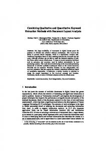
2 Running Example The left figure of Figure 1 shows a robot of the RoboCup soccer team of our university [12]. The robot comprises an omni-directional drive, an pneumatic kicker, an Intel-based central PC running Linux and an omni-directional camera system. The omni-directional drive is shown on the right figure. It comprises three Swedish wheels each propelled by a combination of a brush-less DC-motor, a wheel-encoder and a gearbox. Furthermore, the drive comprises all the power-electronics for these three axis and a central micro-controller running the drive’s firmware. The firmware is responsible

COMBINING QUANTITATIVE AND QUALITATIVE MODELS

Figure 1: An autonomous robot of our RoboCup soccer team on the left. On the right the omni-directional drive of the robot is shown. for the synchronized control of the wheels according to the commanded motion and the drive’s kinematics. Moreover, the firmware is able to provide observations like encoder ticks or odometry data. Furthermore, the firmware comprises special function which allows the firmware to simulate hardware faults in order to allow diagnosis experiments. Such faults are for instance that a motor becomes stuck. Such a behavior is simulated by a permanent break of the motor. The central PC runs a three-layer control software. It comprises a hardware layer, a continuous layer and an abstract layer. The hardware layer is responsible for the interface to all hardware components. The continuous layer performs any continuous information processing like image processing or reactive control. The abstract layer host the deliberative control in form of planning and reasoning module. The continuous layer is able to provide two different kinds of observations about the robot itself and its environment. The layer either provides processed information like the global position and orientation of the robot and the position of recognized objects or it provides unprocessed sensor data like the optical flow in the camera. The presented robot platform will serve as an example for the diagnosis throughout the remainder of the paper.

3 Quantitative Modeling Figure 2 shows the arrangement of one axis of the drive of our robot. It comprises an omni-directional wheel, a gearbox, a servo-motor and a wheel-encoder. Furthermore, it shows the inputs, e.g., commanded velocity, and the outputs, e.g., drawn current and actual angular velocity, we are able to observe. In order to be able to detect and localize a fault in such an electro-mechanical system we have to model the desired behavior of the system. In general, an abstract qualitative model is not sufficient to model all aspects of such systems which are able to provide useful information for diagnosis. Therefore, we have to model the dynamic of the system for all nominal and all faulty operation modes we want to detect. An approved method

Velocity

Current

Servomotor

Command

Gearbox

Encoder


Figure 2: The arrangement, the inputs and outputs of a single axis of the robot drive example. to model the behavior of such systems are probabilistic hybrid automata. A detailed overview on this technique can be found in [13]. In short a probabilistic hybrid automata is an automata which comprises all nominal and faulty operation modes of the system as discrete states. Moreover, the automata comprises transitions between the modes and probabilities for their occurrence. Furthermore, to each state a model of its dynamics is attached, i.e., difference or differential equations, which describes how the continuous state vector of the system evolves in that particular mode. Figure 3 depicts a simple probabilistic hybrid automata which models the example of Figure 2. P12 ¬ok(M )

ok(M ) P11

P21

ω˙ =

P22

1 ω+u+W τ

(1)

1 ω+W τ

(2)

ω˙ =

Figure 3: A simple hybrid automata modelling a single axis. The upper figure shows the automata with the two modes, nominal and faulty, and their transitions. The lower figure depicts the differential equations for the nominal mode (1) and the faulty mode (2). ω denotes the angular velocity. ω˙ denotes the time derivative of the angular velocity. u denotes the input, the desired angular velocity. W models the process noise. The task of detection and localization of a fault in this case is equivalent to find the most probable operation mode based on observations of the system. The state estimation can be performed by multi-hypothesis tracking. The approach tracks all possible mode sequences over time and estimates how likely these sequences are with respect to the observed input and output sequence. That mode sequence with the highest likelihood captures most probable the true mode sequence. Figure 4 depicts such a simulated diagnosis for a fault in the motor example. The state estimation is probabilisticly done as all


measurements and actions are effected by some level of uncertainty.

Figure 4: Example for a diagnosis of one axis of the robot drive. The upper figure shows the actual velocity and the noisy velocity measurement over time. At time t = 0 s a velocity of 0.1 m/s is requested. At time t = 1 s the requested velocity jumps to 0.2 m/s. The true velocity follows these requests with some delay. After time t = 2 s the motor fails and runs out. The lower figure shows the estimated mode. The mode 1 denotes the nominal mode. The mode 2 denotes the faulty mode. The presented schema is in general used for the modelling of systems like hardware where pure qualitative models are too coarse. The reasoning schema used in here is abductive. Abductive reasoning means that we have a theory T and observations O and S we like to find an explanation E for O. If E is an explanation then T E |= O and S T E 6|=⊥ holds. Abductive reasoning can be done in an abstract logical form and also as shown here as probabilistic state estimation. Obviously, we have to model the behavior of all nominal operation modes and all faulty modes we like to detect.

4 Qualitative Modeling In contrast to the quantitative modelling schema qualitative models use an abstract logicbased model of the behavior of a system in order to be able to detect and localize faults. One advantage of this technique is that only the correct behavior of the system has to be modeled. The principles were originally developed by Reiter and was presented in [14]. The basic idea is to use an abstract model, i.e., horn clauses for efficiency reasons, of the correct behavior of the system and some current observations, i.e., predicates, of the system. If the prediction of the model differs from the observation a contradiction occurred and we have detected a fault. The check for such contradictions can be performed easily by logical inference. So far we only know that a fault has been occurred but we do not


know the root cause of a fault. In general it is not obvious which faulty component is responsible for the observation of a faulty behavior. In order to solve this problem efficiently Reiter proposed its hitting-set algorithm. The idea is to systematically take back assumptions about functioning components until the contradiction is removed. Therefore, the removed assumptions about correct components are an explanation for the faulty behavior. These explanations are called a diagnosis. More details about model-based diagnosis can be found in [7]. In [1] an more convincing modeling schema was presented. The schema eases the modeling of larger systems. The idea is that one only models the correct behavior of smaller components, e.g., gates in integrated circuits, and additionally provides a structural description of the connections and interactions of the components. The advantage is that the behavioral description of the components can be easily reused for other systems and only the structural description has to be adapt to the new system. In the remainder of the paper we follow this schema for the qualitative modeling. We continue with an example which depicts the quantitative modeling. The behavior of one axis of the robot drive in Figure 2 can be qualitatively modeled with the following simple clauses: 1. ¬AB(ENCODER) ∧ ¬AB(MOTOR) ∧ turn(M OT OR) → ok(ticks) 2. ¬AB(MOTOR) ∧ drive(M OT OR) → ok(current) Line 1 specifies that if the encoder and the motor works correct and we command the motor to turn we are able to observe encoder increments. The predicate ¬AB(C ) denotes that a component C is not abnormal meaning that C works as expected. ok(o) denotes that the correct observation o has been made. Line 2 specifies that if the motor works correct and we command the motor to turn we can observe that the motor draws current. Now we assume that the encoder of the motor fails and does not provide any encoder ticks anymore even if the motor turns correct. This observation can be expressed by the following clause: drive(M OT OR) ∧ ¬ok(ticks) ∧ ok(current). If we assume that all components work correct, expressed by the clause ¬AB(ENCODER) ∧ ¬AB(MOTOR) we get a contradiction between the outcome of the model and the observation. We can derive ok(ticks) and ¬ok(ticks) at the same time. This means that we have detected a fault. If we systematically remove assumptions about working components, i.e., change ¬AB(C ) to AB(C ), we are able to find one or more sets of these removed assumption which resolves the contradiction. These sets are the diagnosis of the system and describes the root cause of the detected fault. It has to be noted that the set comprising all components always forms a diagnosis. In the example the set {AB(EN CODER)} resolves the contradiction and is the true root cause of the fault. In general we are interested in diagnosis with minimal cardinality. Because of the fact that this approach tries to maintain consistency the technique is also called consistency-based. In general this consistency-based reasoning is less powerful in comparison to abductive reasoning because the latter is able to derive an explanation for an observation. But models for the consistency-based reasoning in general are simpler to obtain and the reasoning process is less computational expensive.


5 Combine Quantitative and Qualitative Models We presented in the previous sections different modeling and diagnosis paradigms. They differ mainly in the used modeling method (qualitative, quantitative or hybrid) and in their reasoning process (probabilistic state estimation, rule-based systems or logic inference). Furthermore, diagnosis methods can differ in their temporal and diagnosis granularity. Some models may deliver rough diagnosis on a fine temporal granularity for the whole system like there is a general fault in the control software. Other models may be capable to provide a much more specific diagnosis about a limited area of the system like the maximum possible angular velocity of a motor is suddenly limited to some value. This shows that the different methods are capable to cope with different aspects of the system with different qualities. Moreover, in general diagnosis methods provide all explanation which are consistent with the model and the observations or which have a probability above some level. But all this explanations are not necessarily comprise the real root cause of the fault. It similar to the situation when one brings its car to the garage because the motor makes a strange noise. The mechanic there often provides the explanation that this or that component causes the noise. In general the true explanation is among that set but further investigation is necessary. Reconsider the example of the failed motor in Section 4. If we are unable to measure the drawn current both diagnosis {AB(EN CODER)} and {AB(M OT OR)} explain the observed behavior. But if we use a global measurement of the path driven by the robot together with a quantitative model of the kinematics of the robot for all modes we are able to reduced the number of diagnosis the the correct one again. In order to use the advantages of the different diagnosis methods while avoiding the drawbacks we propose to combine the different methods to improve the overall performance of the diagnosis. We believe that beside the better quality of the diagnosis with that approach we are able to handle much more complex systems comprising hardware and software. Figure 5 depicts an overview of an architecture which combines different models for the diagnosis process. M denoted the the qualitative and quantitative models and reasoning modules. O denotes the different observations of the system used as inputs for the different diagnosis processes. The observations may origin from different parts of the system and depict various aspects of the system like continue valued measurements or logical predicates. δ denotes the outcome of these local diagnosis processes. The temporal and diagnosis granularity of these diagnoses can be very different. While one model may deliver a full set of components that may have caused the fault another module may just deliver an estimation about the operation mode of a component. Moreover, the diagnosis output of one model can be used as an input for another model. For instance a quantitative model may provide an input predicate for a qualitative model. All the different diagnoses δ represents a different view on different parts of the system. Moreover, they comprises different knowledge and opinions about the state of the system. Obviously, these different parts of knowledge will be sometime inconsistent and will provide different explanations for an observed faulty situation. In order to increase the overall quality of the diagnosis we propose to combine the


Monitored System

δqual,1

... Mquant,m δqual,m

Mquant,1

Oquant,m

Oquant,1

δqual,1

Mqual,n δqual,n

...

Oqual,n

Oqual,1 Mqual,1

Combining Diagnosis Engine ∆

Figure 5: The figure shows the framework for combining qualitative and quantitative models and diagnosis in order to improve the overall diagnosis ∆. different local diagnosis results to a global one. ∆ in Figure 5 denoted the combined improved overall diagnosis of the system. The combination of such divers models and reasoning methods will increase the quality of the resulting quality of the diagnosis but raises a number of open questions: – Different Temporal Granularity The different models may use observations that come at a very wide range of framerates. A hearth-beat message from a component may be received at a frame-rate of about one Hz while other sensors may provide data at a frame-rate up to several hundreds of Hz. Due to this factor also the different reasoning engines my provide their results on such a wide range of frame-rates. Moreover, extensive logical reasoning or the temporal integration of data in the filtering and tracking methods may cause further delays of the diagnosis in respects to the time the observations were made. Therefore, appropriate methods are required in order to synchronize the local diagnosis to avoid contradictions or inconsistencies. There are very good approaches in sensor fusion which addresses the fusion of (uncertain) information provided at different frame-rates and sampling times [15]. – Different Diagnosis Granularity As described in the previous sections the different models and reasoning methods provides diagnosis on a wide range of semantic granularity. On one hand very general abstract diagnoses are provided. In general they are derived by logic inference from an abstract logic-based model. On the other hand filtering and tracking methods are able to provide informations about a system in very fine resolution such as estimations about the continuous state vector of an system. In general the fusion of information on an abstract symbolic level is much easier. In order to be able to fuse continuous valued information at that level we have to perform symbol grounding


for the that values. Symbol grounding can be done in the easiest case by simple thresholding. The disadvantage of such methods is that one probably throws away useful information obtained by quantitative models. Therefore, methods for a direct fusion of quantitative and/or qualitative methods are needed. – Spatial Distribution Another important issue is that different models may provide diagnosis about different parts of the system. One model may provide a diagnosis about the drive hardware of a robot while another model may provide a diagnosis about the control system of the robot. Due to the fact that often a fault in one component also causes a depending fault in an interacting component sometimes false alarms are raised. In order to improve the quality of the diagnosis we have to combine the output of different models. Therefore, the development of meta-models is necessary in order be able to do this information fusion. There exists work about distributed diagnosis but they use in general the same semantics in the output of the models. Therefore, new more general meta-models have to be developed. – Performance Issues In general the presented diagnosis methods are expensive in terms of computational power and memory. This is a limiting factor if such intelligent methods should be deployed in small embedded systems. Anyway, subsets of these methods have already been deployed to embedded systems in cars for instance. These applications gives up some level of flexibility of the methods and compile their knowledge into simpler structures like decision trees. But in the future models with less demand on computational resource have to be developed.

6 Active Observations In general the observations of the systems are caused by the ordinary operation of the system. The system is performing its task and provides observations about itself. Usually, the diagnosis module has no control about which actions the system is actually to perform and therefore what observations are available at that moment. Furthermore, it might happen that exactly these observations do not contain the necessary information which is needed to do the best possible diagnosis. Assume the following situation. During the movement along a given path some component in the drive fails. Usually, the robot continues it started action until it makes another decision. The diagnosis modules only can rely on the observation produced by that current action. In some case these observations might be not sufficient in order to locate the failed component. Therefore, in some situations it will be desirable that the diagnosis and monitoring system is able initiate actions in order to gather more useful information. In the above example such an action can be a special motion pattern or profile for the motors. Such additional observation can help to reject not plausible diagnosis. The application of such active observation request for additional planning and reasoning capabilities because the diagnosis module has to derive which additional information is useful in order to improve the diagnosis and which action will provide the required information. Furthermore, the system has to take care that these additional actions do not endanger the system or the environment even in the case of an occurred fault. For this


purpose additional models and planning strategies have to be developed. Some work has been done on which measurement to encounter next in model-based diagnosis in order to improve the quality of diagnosis [16]. But so far no active methods have been used.

7 Related Research The Livingstone architecture proposed by Williams and colleagues [6] was used by the space probe Deep Space One to detect failures in the its hardware and to recover from them. The fault detection and recovery are based on model-based reasoning. In [17] and [18] particle filter techniques were used to estimate the state of the robot and its environment. These estimations together with a model of the robot were used to detect faults. The most probable state is derived from unreliable measurements. The advantage of this approach is that it is able to handle non-Gaussian uncertainties of the robot’s sensing and acting as well as uncertainties in its environment. Other approaches which are based on Kalman-filter are only able to account Gaussian uncertainties. Model-based diagnosis also has been successfully applied for fault detection and localization in digital circuits, in car electronics and for software debugging of VHDL programs [1]. In [5] Struss et al. presents an approach for knowledge compilation for a diagnosis system. The model and the reasoning process for the diagnosis of parts of the electronics of a car was condensed to a decision tree. This reduction of the demand for resources allowed them to apply the diagnosis system in an ordinary control unit for cars. Roos described in [19] an algorithm which allows a group of diagnosis agents to negotiate a decision about a global diagnosis. The agents had only a local view of the system. The main issue of this work was to minimize the communication overhead needed for a global diagnosis. In [16] a method was presented which is able to decide which measurement should be done next in order to gather maximum information for the diagnosis. The development of this method was mainly driven by the fact that not all measurement contains the same useful information all the time. Furthermore, some measurements are more costly or harder to obtain than others. Therefore, one like to minimize the use of such measurements if possible.

8 Conclusion In this paper we proposed the combination of quantitative and qualitative models and reasoning methods in order to improve the diagnosis capabilities for complex systems comprising hardware and software. Moreover, we presented the properties of quantitative and qualitative diagnosis methods. Based on a running example of an autonomous mobile robot we motivate that such a combination is valuable and how it can be realized. Moreover, we pointed out potential problems and research topics related to the combined diagnosis. These problems mainly concerns the useful fusion of temporal, semantical and spatial divers information. Furthermore, we introduce the idea of active observations which are a way to actively gather additional information for the improvement of the quality of diagnosis. We believe that the proposed framework will influence the achievable quality of supervision. Our future work will be focused in a first step on the fusion of the


divers diagnosis informations.

References [1] Gerhard Friedrich, Markus Stumptner, and Franz Wotawa. Model-based diagnosis of hardware designs. Artificial Intelligence, 111(2):3–39, 1999. [2] Michael Hofbaur, Johannes Köb, Gerald Steinbauer, and Franz Wotawa. Improving robustness of mobile robots using model-based reasoning. Journal of Intelligent and Robotic Systems, 48(1):37– 54, 2007. [3] Gerald Steinbauer and Franz Wotawa. Detecting and locating faults in the control software of autonomous mobile robots. In 19th International Joint Conference on Artificial Intelligence (IJCAI-05), pages 1742–1743, Edinburgh, UK, 2005. [4] Daniel Köb and Franz Wotawa. Introducing alias information into model-based debugging. In Ramon López de Mántaras and Lorenza Saitta, editors, Proceedings of the 16th Eureopean Conference on Artificial Intelligence, ECAI’2004, including Prestigious Applicants of Intelligent Systems, PAIS 2004, Valencia, Spain, August 22-27, 2004, pages 833–837. IOS Press, 2004. [5] Peter Struss and Chris Price. Model-based systems in the automotive industry. AI Magazine, 24(4):17–34, 2004. [6] Nicola Muscettola, P. Pandurang Nayak, Barney Pell, and Brian C. Williams. Remote agent: To boldly go where no AI system has gone before. Artificial Intelligence, 103(1-2):5–48, August 1998. [7] W. Hamscher, Luca Console, and Johan de Kleer, editors. Readings in Model-Based Diagnosis. Morgan Kaufmann, 1992. [8] R. Kalman. A new approach to linear filtering and prediction problems. ASME Transactions, Journal of Basic Engineering, 82:35–50, 1960. [9] B. Anderson and J. Moore. Optimal Filtering. Information and System Sciences Series. Prentice Hall, 1979. [10] R. Isermann. Supervision, fault-detection and fault-diagnosis methods - an introduction. Control Engineering Practice, 5(5):639–652, May 1997. [11] J. Chen and R. Patton. Robust Model-Based Fault Diagnosis for Dynamic Systems. Kluwer, 1999. [12] Gerald Steinbauer, Mathias Brandstötter, Martin Buchleitner, Stefan Galler, Simon Jantscher, Gerald Krammer, Martin Mörth, Jörg Weber, and Martin Weiglhofer. Mostly Harmless Team Description 2006 - Robust Control of Mobile Robots. In Proceedings of the International RoboCup Symposium, 2006. [13] Michael Hofbaur. Hybrid Estimation of Complex Systems, volume 319 of Lecture Notes in Control and Information Sciences. Springer Verlag, 2005. [14] Raymond Reiter. A theory of diagnosis from first principles. Artificial Intelligence, 32(1):57–95, 1987. [15] L. Drolet, F. Michaud, and J. Cote. Adaptable sensor fusion using multiple kalman filters. In Proceedings IEEE/RSJ International Conference on Intelligent Robots and Systems (IROS), 2000. [16] Johan de Kleer. Getting the probabilities right for measurement selection. In 17th International Workshop on Principles of Diagnosis (DX-06), pages 141–146, Penaranda de Duero, Burgos, Spain, 2006. [17] Richard Dearden and Dan Clancy. Particle filters for real-time fault detection in planetary rovers. In Proceedings of the Thirteenth International Workshop on Principles of Diagnosis, pages 1 – 6, 2002. [18] Vandi Verma, Geoff Gordon, Reid Simmons, and Sebastion Thrun. Real-time fault diagnosis. IEEE Robotics & Automation Magazine, 11(2):56 – 66, 2004. [19] N. Roos, A. ten Teije, A. Bos, and C. Witteveen. Multi-agent diagnosis with spatially distributed knowledge. In Proceedings of the Belgium-Netherlands Artificial Intelligence Conference (BNAIC), pages 275–282, 2002.