PSYCHOMETRIKA--VOL. 67, NO. 4, 5 8 9 - 6 0 8 DECEMBER 2 0 0 2
C O M B I N I N G S T A N D A R D I Z E D M E A N D I F F E R E N C E S U S I N G THE METHOD OF MAXIMUM LIKELIHOOD KE-HAI YUAN UNIVERSITY OF NOTRE DAME BRAD J. BUSHMAN IOWA STATE UNIVERSITY A maximum likelihood procedure for combining standardized mean differences based on a noncentral t-distribution is proposed. With a proper data augmentation technique, an EM-algorithm is developed. Information and likelihood ratio statistics are discussed in detail for reliable inference. Simulation results favor the proposed procedure over both the existing normal theory maximum likelihood procedure and the commonly used generalized least squares procedure. Key words: noncentral t-distribution, data augmentation, EM-algorithm, observed information, MonteCarlo, meta-analysis, effect size, maximum likelihood, weighted least squares.
1. Introduction As the number of scientific studies continues to grow at an exponential rate, it becomes increasingly important to integrate the results from these studies. It is somewhat ironic that the traditional review of scientific research has been conducted in an unscientific fashion. In the traditional narrative (qualitative) review, the reviewer uses "mental algebra" to combine the findings from a collection of studies, and describes the results verbally. Narrative reviews are particularly susceptible to the subjective judgments, preferences, and biases of a particular reviewer's perspective. Statisticians were the first to advocate a more scientific approach to reviewing the literature--an approach based on quantitative methods. These quantitative methods were labeled meta-analysis by Glass (1976): Meta-analysis refers to the analysis of a n a l y s e s . . , the statistical analysis of a large collection of analysis results from individual studies for the purpose of integrating findings. It connotes a rigorous alternative to the casual, narrative discussions of research studies which typify our attempts to make sense of the rapidly expanding literature.
(p. 3) In the meta-analytic (quantitative) review, the reviewer uses statistical procedures to integrate the findings from a collection of studies, and describes the results using a numerical effect-size estimate (e.g., Wang & Bushman, 1999). An effect size provides a numerical measure of how strongly two variables are related (e.g., viewing violence and behaving aggressively, smoking tobacco and getting lung cancer). When the primary studies compare two groups, either through experimental (treatment) versus control comparisons or through planned contrasts, the effect size estimate is expressed as some form of standardized difference between group means. This article focuses on estimating the population standardized mean difference. Hedges (1980) proposed using the method of maximum likelihood for estimating the standardized mean difference. His estimate is based on the normal density functions for the experimental and control Requests for reprints should be sent to Ke-Hai Yuan, Laboratory for Social Research, 919 Flanner Hall, University of Notre Dame IN 46556. E-Mail:
[email protected] 0033-3123/2oo2-4/2ooo-o814-A $00.75/0 @ 2002 The Psychometric Society
589
590
PSYCHOMETRIKA
groups. Because of many nuisance parameters involved in this likelihood function (in addition to the mean difference of interest), the resulting estimator may not be consistent even when many studies are combined (Hedges & Olkin, 1985). Consequently, most meta-analyses use a weighted least squares estimator. In this article we propose an alternative maximum likelihood estimator based on the noncentral t-distribution. First, we briefly review the commonly used weighted least squares (WLS) method (Hedges, 1982), and the normal theory based maximum likelihood method (Hedges, 1980, 1982). Next, we describe an alternative method for estimating the standardized mean difference. Suppose that the data for a meta-analysis arise from a series of k independent studies, each of which compares a treatment or experimental group (e) with a control group (c). Let Yeij and Ycij denote the j-th observations in the experimental and control groups of the i-th study, and let nei and nci be the experimental and control group sample sizes. Then it is typical to assume Yeij ~ N(l~ei, a2), j = 1 . . . . .
nei;
and
Ycij ~ N(l~ci, a2), j = 1 . . . . .
nci.
(1)
Let nei Yeij Yei = ~ - ~ , j = l flei 2
nci Ycij Yci = ~ - ~ , j = l flci
nei (Yeij -- Y e i ) 2,
sei-- ~ j=l
L;--i-
2
and
nci (Ycij -- Yci)2
s~i= ~ j=l
~;--~
.
Glass (1976) proposed a simple approach of combining standardized mean differences 3i = (l~ei -- I~ci)/¢r i . Define the pooled estimate of variance as s~ = (nei - 1)s2ei + (nci - 1)S2ci flei ÷ flci -- 2
the standardized mean difference 3i can be estimated by "~ei -- "Yci
di -
-
-
,
(2)
si
however, di is well known a biased estimator of 3i. Hedges (1981) proposed an unbiased estimator of 3i, d~/ = c(pi)di,
(3)
where c(pi) = F ( p i / 2 ) / { ~ F [ ( p i - 1)/2]} and Pi = nei + nci - 2. Hedges (1982) further proposed combining effect sizes using the method of WLS. When the combined sample size is large (i.e., Pi is large), Hedges (1982) suggested the following approximation to the distribution of d/U: d~/ ~ N(3i, ai2(3i)),
(4)
where -
nei
+
neinci
+
.
2(nei ÷ nci)
Let Cp = 1
3 4p - 1'
591
KE-HAI YUAN AND BRAD J. BUSHMAN
then
c(p) ~ cp. Substituting Cp~ for c (pi) in (3) yields the commonly used procedure given by Hedges (1982) for combining standardized mean differences
3veLs - ~,~=1 wid~
Var(~WLS)--
with
k ~ i = 1 wi
1 k ' ~ i = 1 wi
(5)
where wi = 1/a/2(d/U). The estimator ~wLs is used to estimate the common effect size 3 under the null hypothesis Ho :
31 . . . . .
3k = 3.
(6)
It is easy to see that the solution 3WLS corresponds to minimizing the WLS function k
0(3) = ~-~wi(d? - 3) 2. i=1
Hedges (1982) and Rosenthal and Rubin (1982) independently proposed the test statistic Q(~wLs) for testing the null hypothesis given in (6). Under the null hypothesis, Q(3wLs) X2-1"
According to classical statistical theory, the maximum likelihood approach is usually preferred over the WLS approach, unless the data are nonnormally distributed. The advantages of the maximum likelihood estimator (MLE) are that it is asymptotically most efficient and its distribution is easily obtained. Furthermore, the likelihood ratio statistic asymptotically follows a chi-square distribution. These properties are well known (e.g., Stuart & Ord, 1991) and are lacking for other type of estimators. In order to obtain a M L E for 3, Hedges (1980, 1982) formulated the following statistical model for the effect size 3 under the null hypothesis in (6):
Yeij = 3o'i q- ?'i q- ~eij, Ycij = ?'i q- ~cij,
j = 1. . . . . nei,
j = 1. . . . . nci.
(7a) (7b)
2 -2 for model (7), a M L E of 3 can be obtained by Based on the sufficient statistics (Yei, Sei, Yci, Sci) solving k [ ni ('Yei -- Y c i ) 22 1 3k+ ~ - ~ s i g n [ ( Y e i - Y e i ) ] f i 2 ( Y e i - Y e i ) 2 ( 3 2 + g i ) l / 2 = O , ~-~fii i=1 hi i=1 hi
(8)
which is Equation (4.3) of Hedges (1980), where fii = nci nei / (nci + nei),
hi
=
pis2 q_ ~i(Yei
- -
-- Yci)
2
and
4(nci + nei)ai gi -- ~2(Yci _ Yei)2
However, as discussed in Hedges and Olkin (1985), there are two major disadvantages with the MLE based on model (7). First, with a single effect size the MLE d~ = x / ~ + 2di/x/P7 is positively biased. Second, the MLE based on model (7) may not be consistent if neij and ncij remain small even when k --+ oc. This is because the number of nuisance parameters (ai, Vi) increases as k increases (Neyman & Scott, 1948). Due to these two disadvantages, one might wonder whether the MLE based on model (7) is the best estimator. As we shall see, simulation results show that the estimator obtained by solving (8) is positively biased even when k is fairly large.
592
PSYCHOMETRIKA The likelihood function formulated through model (7) contains nuisance parameters
(Vi, ~ri). If a likelihood function can be derived that does not contain nuisance parameters,
then the Neyman-Scott type of problems associated with M L E can be resolved• The positive bias associated with d~ can also be resolved if a proper model for 3 based on model (1) can be derived• The objective of this paper is to develop an approach for a M L E of 3 using a different model formulation• If m i = [neinci/(nei + nci)] 1/2, then under models (1) and (6) we have (9)
xi = m i d i ~ tp~ (Li),
where Li = m i 3 . It is obvious that besides 3 there is no other unknown parameter in the density function of the noncentral t-distribution in equation (9). Thus, the M L E based on model (9) avoids the drawbacks associated with the M L E based on model (7). As we shall see, the M L E based on model (9) also possesses nice small sample properties and is a competitive alternative to 3 w L s . Of course, the density function of a noncentral t-distribution is much more complicated than is the density function of a normal distribution. However, by using proper data augmentation and applying an EM-algorithm, one can obtain the M L E based on model (9) without any numerical difficulty• In section 2 we describe an EM-algorithm based on data augmentation• In section 3 we discuss inference issues regarding the population standardized mean difference. In section 4 we describe the results of a simulation study that compares estimates based on the three methods• In section 5 we present some empirical evidence regarding the convergence of the EM-algorithm and the stability of the three estimators when an extreme effect size is included• In section 6 we discuss the EM-algorithm and offer some conclusions• 2• Data Augmentation and EM-Algorithm If y ~ N()~, 1) and u ~ Xp, then we can write x ~ tp ()~) as
y,/7 Xm
In a meta-analysis, x is observed, but y and u are not observed• We will call y and u latent variables. In order to develop an EM-algorithm for estimating )v, the observed data x are augmented with the latent variable u. Because the conditional distribution of x given u is (xlu) ~ N
,
,
the augmented likelihood function is
uP l ( L l x , u) = f ( x l u ) f ( u )
= 2p/2_lF(p/2)
u2
2x/~~ exp
With a single effect size, our aim is to derive an estimator tion
2
u2 (x - ) w / ~ / u ) 2 2p
~MLthrough
l(~lx) : maxl()qx)•
•
(10)
,~ that satisfies the condi-
(11)
However, the form of the likelihood function l()v Ix) for a noncentral t-distribution is so complicated that a direct solution to equation (11) is formidable if not impossible• An EM-algorithm offers an alternative and easy to implement approach to solve for ,~• The EM-algorithm was first proposed by Dempster, Laird and Rubin (1977), and it has been used in a great number of statistical applications (e•g•, McLachlan & Krishnan, 1997; Tanner, 1996)•
593
K E - H A I Y U A N A N D B R A D J. B U S H M A N
Based on the augmented likelihood function (10), the EM-algorithm is an iterative algorithm consisting of two steps: the E-step and the M-step. Let )~(J) be the current estimate of )~ and let f ( u Ix, )~(J)) be the conditional density of u given x. The E-step is to calculate OG
Q G , )~(J)) =
L
l o g [ f G l x , u ) ] f ( u l x , )~(J))du.
The M-step is to maximize Q with respect to L at L(j+l), treating L(J) as fixed. The process is repeated until I)~(j+l) -)~(J)l is sufficiently small. Before giving more details of the EM-algorithm, we want to point out that the M L E ~ML defined using (11) is different from d~ = x / ~ + 2 d i / x / ~ for a single standardized mean difference. This can be illustrated using an example.
Example 1. Let 3 = (#e - #c)/C~ be a single standardized mean difference. Let ne = nc = 5. Suppose we observe d = 1.0, where d is defined in equation (2). Then x = (5/2) 1/2, and the M L E based on model (7) is d I = x/~-/4 ~ 1.118; 3WLS = .903; and the M L E defined using equation (11) is ~ML= 1.028. The likelihood function l(3 Ix = x/~/2) of x ~ tl (x/~-/23) is a concave function of 3 as can be seen in Figure 1. Suppose a meta-analysis includes k effect sizes. Following the notation used in (9), the observed data are x = (xl, . . . , xk)'. Each xi follows a noncentral t-distribution with degrees of freedom Pi and noncentrality parameter Li = mi3. Let ui be a chi-distribution with degrees of freedom Pi, where the ui, i = 1 . . . . . k are independent. If u = (ul . . . . . uk) I, then our augmented data are (x, m . After dropping a constant term, the joint log likelihood function of
I
I
I
I
I
I
0.3
i i
"C) 0 0 0.2 t-
i !
/ l i
i
0.1
0.0
l.
I
I
I
I
I
I
-4
-2
0
2
4
6
delta FIGURE 1. Likelihood function of noncentral t-distribution with degrees of freedom 8, observed x = (5/2)1/2 and noncentrality parameter (5/2) 1/2(].
594
PSYCHOMETRIKA
(x, u) is k
If
k
-- ~
~2
x2 -}- !Oi. 2 -}- ~ Xi"imi3 i=1 2pi i=1 x/~7
//(3Ix , U)=
u} j) = E(ui Ixi, 3(J)),
then the
k
k
2 ~-]m2 + ~-]piln(ui). i=1
(12)
i=1
EM-algorithm for obtaining ~ML = 3(00) is given by
ximi u(J) 3(j+1) _ ~]/k=l ~
k E,=lm
i
(13)
At each iteration one calculates /~i " (j) ' which is the conditional expectation of ui given (xi, 3(J)). After simplification, the conditional density function of ui given (xi, 3(J)) can be written as
fi(uilxi, 3 (j)) = CiUpi
exp
{
2pi
ui
~7~i)
_] J
with
ci-: u exp/1
ui xi mi+ J'12/ x ui.
(14)
Various numerical approaches are available for evaluating
• (J)
#
ui fi (ui Ixi, 3(J))dui •
(15)
But with the appropriate statistical software, one does not need to actually evaluate these integrals in (14) and (15). Notice that the integrals in (14) and (15) are of the form
Ap(a, b) =
F
u p e x p [ - a ( u - b)2]du.
(16)
When b > 0, using substitution u - b = v we have
Ap(a, b) = Apl(a, b) + Ap2(a, b), where
Apl (a, b) =
#
(v + b) p exp(-av2)dv,
Ap2(a, b) =
F b
(v + b) p exp(-av2)dv.
Further calculation leads to 1 p
Apl(a, b) = ~ ~
F ( p + 1) b (p-q) (q~l) F(q + 1)F(p 7 q + 1) a ~ F - -
'
and 1 ~-](_l)q
Ap2(a, b) = ~
q=O
F ( p + 1) b (p-q) [ ab2 v(q-1)/2e-Vdv" F(q + 1)F(p 7 q + 1) a(V+l)/2 ao
(17)
595
K E - H A I Y U A N A N D B R A D J. B U S H M A N
Almost every statistical software package includes the gamma function. The integral in (17) can be calculated using the incomplete gamma function that exists in both SAS and MATLAB software. For example, denote the incomplete gamma function Fin(S, l ) - - F (1 S)
fot
x~-le-Xdx'
(18)
then
fo ab2 v(q-1)/2e-Vdv
= F
( q- ~- l )
Fin
(qq~l,ab2) - -
(19)
It follows from (17) and (19) that 1~-],(_1) q
Ap2(a, b)
q=0
F(p+e) b(p-q)~ (q~_e)__ F i n { q + e r ( q + 1 ) r ( p - q + 1) a,~ , *,,~r ~,~--'
ab 2)
If c = - b when b < 0, then we have
Ap(a,
b) = yp- ] , ( - l ) (p-q) F ( p + _1) q=o F(q + 1)F(p q + 1)
f oo v(q_l)/2e_~dv.
cp - q
a(q+l)/2 c2
Using the incomplete gamma function (18) we have p
Ap(a, b)
K-,
_l~(p_q)
q=oZ-'~
~
F ( p + 1) F(q + 1)F(p - q + 1)
If ai = (x 2 + pi)/(2pi)
and
- -cFp-q (qq2~l)[1-Fin(q~l,ac2)l. a(q+1)/2
bij = xi~/Tdmi3(J)/(x2 + Pi), then
we can express
u(j) __ Api+l (ai, hi j) i Ap~ (ai, hi j)
(20)
Equations (13) and (20) give the EM-algorithm for obtaining ~ML without difficulty using any program that includes the gamma and incomplete gamma functions. 3. Information and Likelihood Ratio Statistic One advantage of the MLE is that its asymptotic distribution can be characterized by the associated information 2-. In the present context, 2- is given by the negative expectation of the second derivative of the log likelihood function (12). Specifically, the v in (&Me -- 30) ~£ N(0, v)
(21)
is given by 2 - - 1 In the EM-algorithm, the information 2- is not a default output. One has to specifically calculate it. There are several approaches to calculate an information at the convergence of an EM-algorithm (e.g., McLachlan & Krishnan, 1997). The direct evaluation of the second derivative of the likelihood function appears to be the best approach. Denote
gi(ui)
= exp
ui
(~/2+77/)_ ]
,
and
Ai(3) =
uP*gi(ui)dui.
Then, after omitting a constant, the log-likelihood function of (9) can be written as
Ill(a)
--
pim2&2 Pi) + ln[Ai(3)].
2(x/2 +
(22)
596
PSYCHOMETRIKA
For convenience we will use dots on top of a function to denote a derivative. It follows from (22) that
i?~(3)-
2 pim
+
(x 2 + Pi)
)/~ (3) _ _
A~(3)
ai (3)
A/2(3) '
(23)
where Ai
(8)
ximi x/~7
--
u pi+l
foo°°
"u gi( i)dui
x2m23 x2 + p i
foo°°
uPigi (ui)dui,
and
= L (xP +
xy + p,
x~m~3 2 x/-fiT(x 2 + Pi)
upi+,gi(ui)dui + x2m 2 Pi
Let ai = (x 2 + pi)/(2pi) and bi = xix/pTmi3/(x 2 + Pi). Then with we have , " hi) Ai(3) = xx/i m i Api+ltai,
upi+2gi(ui)dui"
Ap(a, b) as defined in (16)
xm>
- -+ p i A p i ( a i , b i ) , x2
and
x4m432
~i(3)=
(x2+pi)2
x2m 2 l A p i ( a i , b i ) _ 2
x2+p ~
x~m~3
Api+l(ai, bi)
v~7(x~ +p~)
+ x2m2Api+2(ai, bi). Pi Evaluation of the information 2-, = - i l (~ML) is tedious but straightforward. Notice that k
27 = - ~
ill (3Me)
(24)
i=1
is the observed information, which is generally more accurate for describing the distribution of ~ML in (21) (Efron & Hinkley, 1978). Before continuing our discussion on information we use an example to illustrate the roles of ne and nc in 27.
Example 2. This example compares the information when ne is fixed and nc increases versus the information when both ne and nc increase. For simplicity, we assume the observed standardized mean difference d = 1.0. With ne = 5, the informations with a single effect size corresponding to values of nc from 5 to 145 are plotted in Panel 1 of Figure 2. The corresponding informations for ne = nc from 5 to 75 are plotted in Panel 2 of Figure 2. As can be seen from Panel 1 of Figure 2, when ne is fixed the information increases as nc increases, but the gain of extra information is diminishing. On the other hand, the information increases linearly as ne = nc increase (see Figure 2, Panel 2). In contrast to the M L E based on model (7), which may not be consistent as k ---> oc (Hedges & Olkin, 1985), t h e ~ML based on model (9) approaches 30 as k --+ oc even when t~ei and nci are small. This can be established under fairly standard conditions (see Yuan & Jennrich, 1998). However, one does not need to assume that k approaches infinity in order for the result in equation
KE-HAI i
i
i
f {1) ..I3
i
i
i
i
f
4.5
{1) ..{3
¢" O
i
i
i
i
i
i
3O
ff
~: 4.0 c
597
Y U A N A N D B R A D J. B U S H M A N
c= 20
3.5
c 0
3.0
.filo
O
"E 2.5
c-
o
2.0
3'0 5'5 8'0 16s 1;o lss
313 5'5 8'0 165 130 155 degrees of freedom
degrees of freedom
Panel 1: ne = 5, nc = 5-145, d = 1.0
Panel 2: ne = nc = 5-75, d = 1.0
FIGURE 2. Information versus degrees of freedom•
(21) to hold. This is because 2-i can be quite large when ne and nc are large enough, as illustrated in Example 2. Actually, one can write (21) as X / Z ( 3 M L -- 30) ~
N(0, 1).
(21a)
The 2- in equation (21a) plays the role of sample size. As long as 2- is large enough, the result in (21) will yield a reliable inference. For a single effect size, this is illustrated in the following ;(old) example. From now on, we will denote the MLE defined in (8) Dy O M L and the one defined in ,~(new) (11) bY~ML " • • • ~(new) E x a m p l e 3. This example illustrates the distribution of 3ML a s the information increases. ~(new) We choose 3 = 1.0, ne = nc = 10, 20, 40, 80. For a single effect size, the estimates ~ML based
on 500 simulation replications are plotted in Figure 3 using quantile-quantile (QQ) plots. Notice ~(old) and 3 w L s are multiples of the two-sample t-statistic, so they that, with a single study, both ~ML approach a normal distribution quickly. We also have the QQ plots of the corresponding 3 w L s Ae ~(old) for comparison purposes, and the QQ plots ut OML are identical to those of 3 w L s . As reflected ~ ( n e w ) and 3 w L s are quite similar, both approach normality by the QQ plots, the distributions of ~ML as sample size increases. However, there are important differences between the three estimators that we will describe in section 4. Let/3 = (31 . . . . . 3k) I, where each 3i is a free parameter. Then/3 represents the most general alternative hypothesis against the Ho in (6). It is easy to see that/3(3) = (3 . . . . . 3) I corresponds to the null hypothesis, which is nested within/3. Based on this nesting, the likelihood ratio test statistic T L R for Ho is TLR h(new) = ;~(new)
=
~(new)ai
2[ll
~(new) )], (t~ (new) ML)--ll(3ML ~(new)
(25)
where ~'ML ' ~ I M L , " " " , ~ k M L J and ~iML is the MLE of 3i based on the i-th study. It is well known that a likelihood ratio statistic approximately follows a chi-square distribution when ,~(new) the sample size is large enough. Because the TLR in (25) involves each ~iML that only depends on data from the i-th experiment, we need to have all the 2-i large in order for the TLR to be well approximated by Zff_v Similarly, the Zi needs to be large in order for the TLR to be well approximated by a noncentral chi-square when (6) does not hold.
Maximum Likelihood
Weighted Least Squares ,~t--
_.J
~o
co o •.~ CXl
o I
o
-'4
-'2
6
i-
~
-4
-2 0 2 normal quantiles
normal quantiles
(a) ne = 10, nc = 10, 3 = 1 Maximum Likelihood
Weighted Least Squares
L.~ £xl. .J
~o-
~0.
o -2
0 normal quantiles
-2
2
(b) n e = 2 0 , n c = 2 0 , 3 =
b normal quantiles
1
Maximum Likelihood
Weighted Least Squares
,~t-._E -g c4
.~cJ-
co O-
o -2
0 2 normal quantiles
-2
4
6 2 normal quantiles
(C) n e = 4 0 , n c = 4 0 , 3 = 1 Weighted Least Squares
Maximum Likelihood
(N.
~o.
o. -o
"o o -2
0
-2
2
normal quantiles
0
2
normal quantiles
(d) n e = g 0 , n c = 8 0 , 3 = FIGURE 3.
1
~(rzew) and gWL5 based on a single effect size with 500 replications.
Normal probability plots for ~ M L
598
4
KE-HAI
599
Y U A N A N D B R A D J. B U S H M A N
4. Simulation Study When sample size is large, the m a x i m u m likelihood method developed in section 2 has the advantage of yielding the most efficient parameter estimates for large sample sizes. One may wonder whether there is any advantage for the ~ML
with small to medium sample sizes. We
~(new)
~(old)
will compare the finite sample properties of the ~ML with those of ~ML and 3wLs. We will focus on bias and efficiency for the three types of estimators. In the simulation design we choose: 3o = .1, . 2 , . . . , .9. Virtually all meta-analyses have found effect sizes in this range (Hedges, 1982). Based on empirical research, Cohen (1977) proposed 3o = 0.20, 0.50, and 0.80 as small, medium, and large effects, respectively. So our effect size selection covers small to large effect sizes. The numbers of independent studies (k) in the meta-analysis were k = 24, 40, and 67. We obtained these values o f k by counting the number of studies included in 390 meta-analytic studies published in Psychological Bulletin through the year 2000. The value k = 24 is the 25th percentile for these 390 meta-analyses, the value k = 40 is the 50th percentile, and the value k = 67 is the 75th percentile. The average sample sizes per group were 5, 10, 20, 50, and 100. Because not all sample sizes in the experimental and control groups are equal in typical social science research, we let nei and ncz be generated using n = [N x U] + 2, where U is a random variable that follows the uniform distribution
TABLE 1. ~ . "~
~(old)
Bias, standard deviation, a n d coefficient of variation ~1 o W L S , O M L
. "~(new)
ana OML
(Average sample sizes n e = 5, n c = 5)
~(old) ~ML
~WLS
,a(new) OML
k
8
biasxl03
SD
CV
biasxl03
SD
CV
biasx 103
SD
CV
24
.10 .20 .30 .40 .50 .60 .70 .80 .90
-2.712 -22.073 -32.652 -48.001 -41.341 -64.384 -75.046 -80.952 -104.206
0.122 0.127 0.136 0.127 0.132 0.134 0.131 0.145 0.149
1.250 0.712 0.507 0.361 0.288 0.250 0.210 0.201 0.187
18.742 25.554 29.808 36.736 54.550 62.875 57.995 90.350 94.318
0.150 0.160 0.166 0.156 0.160 0.167 0.160 0.179 0.187
1.259 0.709 0.502 0.357 0.288 0.252 0.211 0.202 0.188
8.847 3.426 0.799 -2.839 10.211 4.174 -3.819 9.959 1.340
0.136 0.144 0.152 0.142 0.147 0.151 0.146 0.163 0.169
1.252 0.710 0.504 0.359 0.288 0.251 0.210 0.201 0.187
40
.10 .20 .30 .40 .50 .60 .70 .80 .90
-11.379 -29.649 -27.837 -34.102 -52.478 -63.726 -73.503 -95.370 -108.610
0.103 0.101 0.103 0.096 0.105 0.106 0.099 0.108 0.105
1.167 0.593 0.377 0.261 0.236 0.198 0.159 0.153 0.133
9.495 11.034 32.705 47.180 50.543 71.526 66.287 75.323 88.462
0.127 0.125 0.125 0.117 0.130 0.134 0.122 0.136 0.132
1.157 0.594 0.377 0.262 0.236 0.199 0.159 0.155 0.133
-0.238 -7.731 4.620 9.592 2.427 8.543 1.234 -4.488 -3.702
0.116 0.114 0.115 0.107 0.118 0.121 0.111 0.123 0.119
1.160 0.593 0.377 0.261 0.235 0.199 0.158 0.154 0.133
67
.10 .20 .30 .40 .50 .60 .70 .80 .90
-12.370 -20.635 -28.771 -46.587 -55.304 -67.313 -75.030 -87.295 -105.175
0.078 0.078 0.079 0.079 0.077 0.075 0.082 0.077 0.083
0.888 0.437 0.289 0.223 0.173 0.141 0.132 0.109 0.104
9.238 19.217 31.213 38.438 50.483 59.897 71.109 77.341 96.724
0.098 0.096 0.096 0.099 0.095 0.093 0.102 0.096 0.104
0.893 0.439 0.290 0.225 0.173 0.140 0.133 0.109 0.105
-0.854 0.706 3.390 -0.900 1.085 0.812 2.974 0.501 1.951
0.088 0.088 0.088 0.089 0.086 0.084 0.093 0.087 0.094
0.891 0.439 0.290 0.224 0.173 0.140 0.132 0.109 0.104
600
PSYCHOMETRIKA
on (0, 2), and [N × U] is the integer part of N x U. On average, nei = nci = N + 2 but the experimental and control group sample sizes generally are not equal for a specific experiment. For each c o m b i n a t i o n of 30, k, nei and nci, 500 replications w e r e performed. Let 3r denote an effect size estimate in the rth replication, the bias and variance w e r e calculated respectively as 500 (& _ g)2 bias=a-30,
and
var=~
50()
'
r=l w h e r e 3 z z-.-,r v ' 5 °=° 1 3 r / 5 0 0 . The results corresponding to average sample sizes 5, 10, 20, 50, 100 are reported in Tables 1 to 5, respectively. F r o m these tables, and m o r e simulation conditions that are not presented here, w e notice that the 3WLS is essentially always negatively (or systematically) ~(old) is essentially always positively (or systematically) biased. The amount biased whereas the ~ML of bias appears smaller with larger ne and nc but does not decrease w h e n k increases. In contrast, ~(new) A_ ~(old) the bias in ~ML is m u c h smaller. Actually, unlike the biases in either 3WLS u, OML , the biases in ~ML alternate b e t w e e n positive and negative. Thus, the bias an OML m a y not be systematic. ~(new) Equation (21a) implies that there is no systematic bias in ~ML w h e n the information 2- is large.
TABLE 2. "~(new) Bias, standard deviation, and coefficient of variation of gWLS, g~l~) and" OML (Average sample sizes ne nc = 10)
~(old) ~ML
~WLS
=
10,
a(new) OML
k
8
biasxl03
SD
CV
biasxl03
SD
CV
biasx 103
SD
CV
24
.10 .20 .30 .40 .50 .60 .70 .80 .90
--3.967 --15.236 --15.304 --16.460 --22.400 --37.867 --34.628 --31.310 --49.604
0.096 0.102 0.100 0.103 0.094 0.097 0.089 0.099 0.099
1.000 0.549 0.351 0.268 0.198 0.172 0.135 0.129 0.116
5.267 5.599 11.093 20.793 18.883 18.387 23.041 42.213 40.844
0.105 0.113 0.109 0.113 0.103 0.106 0.098 0.109 0.110
0.999 0.552 0.351 0.268 0.198 0.172 0.135 0.129 0.117
1.116 --3.871 --0.759 4.016 0.372 --6.866 --2.913 8.940 --0.325
0.101 0.108 0.105 0.108 0.099 0.102 0.094 0.104 0.105
0.999 0.550 0.351 0.268 0.197 0.172 0.135 0.129 0.116
40
.10 .20 .30 .40 .50 .60 .70 .80 .90
--7.092 --13.200 --9.215 --14.296 --29.243 --34.039 --30.736 --40.508 --46.634
0.072 0.076 0.077 0.071 0.078 0.077 0.072 0.075 0.077
0.779 0.406 0.266 0.184 0.165 0.136 0.107 0.099 0.091
1.999 5.258 17.345 21.318 15.202 26.938 30.750 34.885 39.959
0.079 0.084 0.084 0.077 0.085 0.085 0.078 0.083 0.085
0.779 0.407 0.265 0.184 0.165 0.136 0.107 0.099 0.091
--2.087 --3.079 5.417 5.367 --4.818 --0.717 2.947 0.633 0.531
0.076 0.080 0.081 0.075 0.082 0.081 0.075 0.079 0.082
0.779 0.407 0.266 0.184 0.165 0.136 0.107 0.099 0.091
67
.10 .20 .30 .40 .50 .60 .70 .80 .90
--6.856 --11.073 --15.905 --24.176 --21.694 --27.182 --39.908 --39.372 --51.968
0.057 0.061 0.059 0.059 0.059 0.057 0.057 0.058 0.064
0.610 0.321 0.208 0.158 0.124 0.100 0.086 0.077 0.075
2.564 6.404 10.017 14.260 25.129 28.677 24.719 33.426 35.179
0.063 0.066 0.064 0.066 0.065 0.063 0.063 0.064 0.070
0.610 0.320 0.207 0.159 0.124 0.100 0.086 0.077 0.075
--1.686 --1.445 --1.608 --3.104 3.975 3.388 --4.577 0.459 --4.501
0.060 0.064 0.062 0.063 0.063 0.060 0.060 0.062 0.067
0.610 0.320 0.207 0.158 0.124 0.100 0.086 0.077 0.075
601
KE-HAI YUAN AND BRAD J• BUSHMAN TABLE 3. Bias, standard deviation, and coefficient of variation of 8WLS,
"ML~'(°ld) (Average sample sizes ne = and "ML~'(new)
20,
nc = 20) ~(old)
~WLS
~(new)
~ML
dML
k
8
biasxl03
SD
CV
biasxl03
SD
CV
biasx 103
SD
CV
24
.10 .20 .30 .40 .50 .60 .70 .80 .90
0.112 -5.700 -8.072 -15.086 -9.398 -14.866 - 14.799 -23.312 -18.519
0.070 0.069 0.065 0.076 0.073 0.070 0.065 0.070 0.075
0.695 0.356 0.223 0.198 0.149 0.119 0.095 0.090 0.085
4.442 4.473 4.528 2.250 10.214 11.531 11.865 10.810 24.910
0.073 0.073 0.068 0.080 0.076 0.073 0.068 0.073 0.079
0.696 0.356 0.223 0.198 0.149 0.119 0.095 0.090 0.086
2.540 -0.025 -1.025 -5.403 1.590 -0.157 0.080 -4.327 5.506
0.071 0.071 0.067 0.078 0.075 0.071 0.067 0.071 0.077
0.695 0.356 0.223 0.198 0.149 0.119 0.095 0.090 0.085
40
.10 .20 .30 .40 .50 .60 .70 .80 .90
-7.254 -4.625 -1.323 -9.392 -10.892 -19.778 -20.831 -19.228 -23.872
0.054 0.056 0.055 0.056 0.057 0.057 0.054 0.054 0.058
0.578 0.286 0.184 0.143 0.117 0.098 0.079 0.069 0.066
-2.916 4.259 11.187 6.845 10.189 8.989 8.002 16.855 17.290
0.056 0.059 0.057 0.058 0.060 0.060 0.056 0.057 0.061
0.577 0.286 0.184 0.143 0.117 0.098 0.079 0.069 0.066
-4.824 0.332 5.688 -0.307 0.899 -3.795 -4.767 0.799 -1.073
0.055 0.057 0.056 0.057 0.059 0.058 0.055 0.056 0.059
0.578 0.286 0.184 0.143 0.117 0.098 0.079 0.069 0.066
67
.10 .20 .30 .40 .50 .60 .70 .80 .90
-1.463 -5.874 -8.341 -10.434 -9.940 -15.887 -17.592 -20.845 -22.257
0.042 0.042 0.040 0.043 0.043 0.043 0.043 0.042 0.043
0.429 0.214 0.137 0.109 0.089 0.074 0.063 0.053 0.049
3.195 2.298 3.778 8.004 12.388 10.211 13.172 13.045 19.374
0.044 0.043 0.042 0.045 0.045 0.045 0.045 0.043 0.045
0.429 0.214 0.137 0.109 0.089 0.074 0.063 0.053 0.049
1.139 -1.300 -1.551 -0.146 2.516 -1.354 -0.479 -2.013 0.811
0.043 0.043 0.041 0.044 0.045 0.044 0.044 0.043 0.044
0.429 0.214 0.137 0.109 0.089 0.074 0.063 0.053 0.049
Empirical standard deviations (SD) of the three estimators for each condition are also reported in Tables 1 to 5• Based on the fact that the SDs for 3wLs are less than those for either ML
u, OML , one may be tempted to conclude that 3wLs is the most efficient one among the
three. In the present context, however, this is a false conclusion. For a parameter estimator (), another estimator g = a() always has a smaller standard deviation when a < 1. This does not imply that g is a more efficient parameter estimator than is (). Comparing SDs is not fair when one estimator is negatively biased. Instead of comparing SDs, we will compare coefficients of variation (CV) as a criterion for efficiency. The CV is given by CV--
SD mean
The CV for ~wLs, ~ML j(old) a~n u OML i(ne~) are reported in Tables 1 to 5. The corresponding CVs suggest that the three estimators are similar in terms of efficiency• Notice in Tables 1 to 5 that the standard deviations decrease when either k or the averaged sample size increases• The standard deviations increase as 30 increases, whereas the coefficients of variation decrease as 30 increases• This can be understood in the following sense: Measuring a larger effect size is easier than measuring a smaller effect size to a certain amount of relative accuracy•
602
PSYCHOMETRIKA TABLE 4.
Bias, standard deviation, and coefficient of variation of
gWLS,g ~ )
"~(neto)
ana" OML (Average sample sizes
ne =
50,
nc = 50)
~(old) ~ML
~WLS k
3
biasxl03
SD
CV
24
.10 .20 .30 .40 .50 .60 .70 .80 .90
-2.520 -2.268 -1.839 -1.505 -5.724 -7.084 -6.696 -6.933 -10.010
0.043 0.046 0.043 0.051 0.042 0.043 0.042 0.047 0.048
0.444 0.235 0.144 0.127 0.084 0.073 0.061 0.059 0.054
40
.10 .20 .30 .40 .50 .60 .70 .80 .90
-0.739 -2.974 -1.773 -5.661 -3.755 -4.938 -5.189 -5.609 -7.732
0.033 0.035 0.035 0.034 0.034 0.036 0.035 0.036 0.036
67
.10 .20 .30 .40 .50 .60 .70 .80 .90
-1.099 -0.485 -2.958 -3.897 -2.544 -4.538 -5.724 -7.448 -7.815
0.026 0.027 0.027 0.027 0.028 0.027 0.027 0.028 0.030
biasxl03
~(new) dML
SD
CV
biasx 103
SD
CV
-0.886 1.729 3.075 5.179 1.810 3.032 3.482 6.284 6.893
0.044 0.047 0.044 0.051 0.042 0.044 0.043 0.048 0.049
0.444 0.235 0.145 0.127 0.084 0.073 0.061 0.059 0.054
-1.595 -0.011 0.941 2.274 -1.463 - 1.390 -0.959 0.498 -0.551
0.044 0.047 0.043 0.051 0.042 0.044 0.043 0.048 0.049
0.444 0.235 0.144 0.127 0.084 0.073 0.061 0.059 0.054
0.336 0.176 0.117 0.086 0.069 0.060 0.050 0.045 0.041
1.036 0.405 2.985 0.576 4.360 6.439 6.049 8.407 8.185
0.034 0.035 0.035 0.035 0.035 0.036 0.036 0.037 0.037
0.336 0.176 0.117 0.086 0.069 0.060 0.050 0.045 0.041
0.266 -1.063 0.921 -2.138 0.832 1.462 1.137 2.260 1.183
0.034 0.035 0.035 0.034 0.035 0.036 0.035 0.036 0.037
0.336 0.176 0.117 0.086 0.069 0.060 0.050 0.045 0.041
0.265 0.134 0.091 0.068 0.057 0.046 0.039 0.035 0.033
0.653 2.692 1.743 3.241 6.147 5.583 6.290 5.632 8.299
0.027 0.027 0.028 0.027 0.029 0.028 0.027 0.028 0.030
0.265 0.134 0.091 0.068 0.057 0.046 0.039 0.035 0.033
-0.107 1.315 -0.296 0.134 2.364 1.164 1.035 -0.103 1.217
0.026 0.027 0.027 0.027 0.029 0.028 0.027 0.028 0.030
0.265 0.134 0.091 0.068 0.057 0.046 0.039 0.035 0.033
5. Examples It is well-known that the EM-algorithm can have a very slow rate of convergence. Accordingly, various acceleration methods have been developed (e.g., Jamshidian & Jennrich, 1993; Louis, 1982; Meilijson, 1989). For some empirical examples presented in chapter 4 of McLachlan and Krishnan (1997) the EM-algorithm may take more than 100 iterations to finally converge while an accelerated procedure takes far fewer (e.g., 11) iterations. In order to understand the convergence of the particular EM-algorithm in (13), we also apply it to several empirical examples. ,~(old) In addition to study the convergence of (13), we also compare the sensitivity of ~wLs, ~ML and
ML
when an extreme effect size exists in the data to be combined. Our data sets are from Tables 6 to 9 of Hedges and Olkin (1985, pp. 23-25), these are respectively the effect of open education on attitude toward school, on student independence and self-reliance, on student self-concept, and on student creativity, with k = 11, 7, 18 and 10 ,~(old) studies collected by Hedges, Giaconia, and Gage (1981). For obtaining ~ML by solving (8), we use the Newton-Raphson algorithm. Using ~wLs as the initial value in both the Newton-Raphson and the EM-algorithms, the number of iterations for convergence are presented in Table 6. Our convergence criterion was chosen a s 1(3 (j-f-l) - 3(J))/3(J) I < 10 -8, where 3 (j) is the value of 3 after the j - t h iteration.
KE-HAI YUAN AND BRAD J. BUSHMAN
603
TABLE 5. (Average sample sizes ne = lee, Bias, standard deviation, and coefficient of variation of gWLS, ~ML~(°ld) and ~ML~(new) nc = lee)
},(old) ~ML
~WLS
~(new) dML
k
3
biasxl0 3
SD
CV
biasxl0 3
SD
CV
biasx 10 3
SD
CV
24
.10 .20 .30 .40 .50 .60 .70 .80 .90
0.485 -0.772 -0.714 -2.601 -4.004 -3.960 -4.703 -3.666 -5.976
0.032 0.033 0.032 0.035 0.030 0.033 0.029 0.033 0.033
0.314 0.166 0.107 0.088 0.061 0.056 0.042 0.041 0.037
1.314 1.183 1.700 0.657 -0.294 1.026 0.286 2.854 2.425
0.032 0.033 0.032 0.035 0.031 0.034 0.030 0.033 0.034
0.314 0.166 0.107 0.088 0.061 0.056 0.042 0.041 0.037
0.957 0.338 0.658 -0.751 -1.899 -1.144 -1.882 0.013 -1.254
0.032 0.033 0.032 0.035 0.030 0.033 0.030 0.033 0.033
0.314 0.166 0.107 0.088 0.061 0.056 0.042 0.041 0.037
40
.10 .20 .30 .40 .50 .60 .70 .80 .90
-0.378 -0.320 -0.491 -1.231 -2.787 -2.499 -3.124 -4.514 -4.587
0.024 0.025 0.025 0.024 0.026 0.026 0.023 0.025 0.026
0.243 0.127 0.085 0.059 0.053 0.044 0.033 0.032 0.029
0.501 1.362 1.842 1.848 1.212 3.127 2.419 2.398 3.248
0.024 0.026 0.026 0.024 0.027 0.026 0.023 0.026 0.027
0.243 0.127 0.085 0.059 0.053 0.044 0.033 0.032 0.029
0.122 0.636 0.835 0.515 -0.518 0.682 0.008 -0.617 -0.179
0.024 0.026 0.026 0.024 0.026 0.026 0.023 0.026 0.026
0.243 0.127 0.085 0.059 0.053 0.044 0.033 0.032 0.029
67
.10 .20 .30 .40 .50 .60 .70 .80 .90
-0.765 0.006 -0.931 -0.807 -1.640 -1.796 -2.715 -4.396 -3.030
0.020 0.019 0.019 0.018 0.019 0.019 0.019 0.018 0.020
0.201 0.096 0.062 0.046 0.038 0.032 0.027 0.022 0.022
0.116 1.563 1.389 2.744 2.644 3.200 3.231 2.018 4.937
0.020 0.019 0.019 0.019 0.019 0.019 0.019 0.018 0.020
0.201 0.096 0.062 0.046 0.038 0.032 0.027 0.022 0.022
-0.264 0.892 0.387 1.207 0.789 1.031 0.643 -0.781 1.453
0.020 0.019 0.019 0.018 0.019 0.019 0.019 0.018 0.020
0.201 0.096 0.062 0.046 0.038 0.032 0.027 0.022 0.022
TABLE 6. Number of iterations for EM-algorithm to converge in four empirical data sets WLS Estimator
Old MLE
No. of Sources 1 Table Table Table Table
6 7 8 9
k 11 7 18 10
~WLS .286 -.097 .011 .054
(.056) (.099) (.042) (.080)
Iterations N/A N/A N/A N/A
New MLE No. of
~(old) ~ML .290 -.100 .010 .061
(.055) (.098) (.042) (.078)
Iterations 3 2 2 3
No. of
~(new) OML .288 -.098 .011 .058
Iterations
(.056) (.099) (.042) (.080)
1Based on the Effects of Open Education as reported in Tables 6 to 9 of Hedges and Olkin (1985, pp. 23-25).
5 5 4 6
604
PSYCHOMETRIKA
The Newton Raphson algorithm for ,~(old) ~ML converges with 3, 2, 2, 3 iterations respectively ~(ne~) converges in 5, 5, 4 and 6 iterations for the four data sets whereas the EM-algorithm for ~ML respectively. Contrasting to the accelerated EM-algorithms reported in McLachlan and Krishnan (1997), the EM-algorithm in the context for combining standardized mean differences in (13) probably will not need any accelerations. Actually, the results in Table 6 were calculated on a PC with a Pentium I1400 processor, which was considered a rather slow computer, and each row was finished instantly. So the slower convergence of (13) is not a serious issue for typical data sets in practice. The convergence of (13) in a few iterations is probably due to the fact that ~wcs is a very good starting value and there is only one unknown parameter 3 involved. In addition to the number of iterations in Table 6, w e have also reported the ~wcs,
ML and ~ML
together with their standard errors. The standard error of ~WLS is given by
~(old) is calculated through the square root of the recip(1/~/k=l wi) 1/2, the standard error of ~ML rocal of the information corresponding to 3 in model (7) as given in Equation (4.7) of Hedges (1980), the standard error of ~MC is calculated according to the one developed in section 3. In the rest of this section w e will illustrate the effect of an extreme effect size on the three ~(old) ^(new) estimators ~wcs, ~MC and 3Me . For such a purpose, w e take the data set in Table 6 of Hedges TABLE 7.
~(new)
The effect of extreme effect size and sample size on gWLS, g~L a)-'' anct OML 1
~,(old) ~ML
~WLS Data
No. o f
6WLS
Iterations
No. o f
~MLo
~(new)
Iterations
No. o f
OML ~MLN
Iterations
.286
N/A
.290
1
.288
5
d12 = 1 2 3 4 5
.287 .288 .289 .290 .290
N/A N/A N/A N/A N/A
.293 .294 .295 .295 .295
3 3 3 3 3
.290 .292 .292 .292 .292
5 5 5 5 5
-1 -2 -3 -4 -5
.284 .282 .282 .281 .281
N/A N/A N/A N/A N/A
.286 .284 .284 .284 .284
2 2 2 2 2
.285 .284 .283 .283 .283
5 5 5 5 5
.296 .306 .325 .363 .435
N/A N/A N/A N/A N/A
.302 .313 .335 .378 .460
3 3 3 3 3
.299 .310 .332 .376 .457
5 5 6 6 7
.274 .262 .239 .193 .106
N/A N/A N/A N/A N/A
.275 .261 .233 .180 .078
2 2 3 3 3
.275 .261 .233 .179 .077
5 5 6 6 7
Original Data
(nel2=ncl2=2)
d12 = 3
nel2=ncl2 = 5 10 20 40 80 d12 = - 3
nel2=ncl2 = 5 10 20 40 80 Based on
EffectsofOpenEducationdata from Table 6 of Hedges
and Olkin (1985, p. 24).
K E - H A I YUAN AND BRAD J. BUSHMAN
605
and Olkin (1985, p. 24) and add an extreme study effect to it. So the total number of studies combined is k = 12 instead of the original k = 11. First, we fix the sample sizes at ne12 = nc12 = 2 while changing the standardized mean difference from d12 = 1 to d12 = 5. All of these values exceed Cohen's (1977) conventional value for a large effect (i.e., d = 0.80). The corresponding changes in the three estimates are shown in the first five rows of Table 7. All three estimators are quite robust to extreme outlier, each only increases by about .005 when adding d12 = 5. A similar pattern of change in the reverse direction can be observed when adding d12 = - 1 to d12 = - 5 , as shown in the next five rows of Table 7. The lower portion of Table 7 contains the result when fixing d12 = 3 and d12 = - 3 while changing sample sizes ne12 = nc12 = 5 to 80. Different from the top portion, each estimator in the lower portion of Table 7 is strongly influenced by the sample sizes associated with the extreme effect size. For example, when ne12 = nc12 = 80 and d12 = - 3 the resulting estimator is less than half of the estimator corresponding to the original data set. When comparing the three estimators, the two M L E ' s have similar reactions to the changing sample size while the reaction of 3 v e c s is, to some degree, less sensitive. When a study has small sample sizes ne and nc, it is likely that the effect size may not be reliable. Of course, outliers are more common in small samples than in large samples (e.g., think of getting 7 heads in 10 coin tosses versus 700 heads in 1,000 coin tosses). When ne and nc are relatively large, we may have to trust the corresponding effect size, although it is in the extreme range. The three methods of combining mean differences, especially the two MLEs, automatically adjust for outliers. So, in practice, we may not need to worry about extreme effect sizes so much if the effect sizes are combined using any of the three methods described in this article. Other more robust alternatives to t h e ~ M L E are discussed in detail by Zhang and Schoeps (1997). Table 7 also contains the numbers of iterations of the Newton-Raphson algorithm and the EM-algorithm, the later one converges within 10 iterations for all the cases.
6. Discussion and Conclusion Since it was introduced by Dempster et al. (1977), the EM-algorithm has been applied to solving many practical problems that the traditional Newton type method cannot easily solve. One of its most important applications is to estimate the mean vector and covariance matrix of a multivariate normal distribution with missing data (Dempster et al., 1977; Little & Rubin, 1987). Rubin (1983) implemented the EM-algorithm for obtaining the means and covariances of a multivariate t-distribution with complete data. Little (1988) extended it to the case of missing data with a multivariate t-distribution of known degrees of freedom. Recently, Liu and Rubin (1995) further extended the EM-algorithm to the case of unknown degrees of freedom for a multivariate t-distribution. In this paper, we extended the EM-algorithm to the one dimensional noncentral t-distribution for estimating the 3 in tp~ (mi 3). Although it has been fully realized that a rescaled version of the sample standardized mean difference follows a noncentral t-distribution, to our knowledge, the estimation of the common 3 by maximizing the density function of a noncentral t-distribution has never been developed. Because the Newton-type method for directly maximizing the likelihood function is unusually complicated, we developed an EM-algorithm method instead. With a program language, the implementation of this algorithm is straightforward. As with any other applications of data augmentations, the value of the EM-algorithm in section 2 lies in its ability to solve complicated problems. This is the beauty of the tool of data augmentation. The advantage of the new M L E is that it is asymptotically efficient. The variance of ~ML is given by the inverse of the associated information, which we discussed in detail in the context of combining standardized mean differences. The likelihood ratio statistic for testing the homogeneity of effect sizes is also straightforward. Compared to the old M L E based on model (7), the formulation of the new M L E does not involve any nuisance parameters and thus ~ML is still
606
PSYCHOMETRIKA
consistent even when the experimental and control group sample sizes are small. The approximation in (4) by Hedges (1982) is based on the assumption that the experimental and control group sample sizes are large in each study. When the experimental and control group sample sizes are small in each study, or even in s o m e of the studies, the approximation in (4) is not very accurate and consequently the value of formula (5) is compromised. The only drawback with the
A_ ~(old)
new MLE is that it needs more computational time than is needed fu, OML o r ~WLS.However, this drawback is not really an issue in this age of modern computers. For example, for any of the 390 meta-analyses published in Psychological Bulletin, it will be an instant to obtain the ~ML on a desktop computer. Notice that the approximation cp of c(p) was used in obtaining the ~wLs. One may wonder if the negative bias in ~WLS is caused by this approximation. Actually, cp > c(p) for every p. Thus, if c(p) is used instead of cp in calculating ~WLS, the bias will be even worse. Of course, the efficiency of the ~WLS will be the same whether cp or c(p) is used. ~(old) In summary, the amount of bias in ~wLs or ~ML increases as 3 increases, it decreases when the average sample sizes ne and nc increase. The bias is insensitive to the number of combined studies k. The new MLE w e propose is less biased than the old MLE and the WLS estimator, especially when the experimental and control group sample sizes are small. Moreover, the minimal bias that does exist in the new MLE is not systematic. Even though the bias in the other two estimators was small, it was systematic. Of course, unbiased estimators are more desirable than biased estimators. Thus, the new MLE should be a valuable tool to the practicing recta-analyst.
References Cohen, J.J. (1977). Statisticalpower analysis for the behavioral sciences (2nd ed.). Hillsdale, N J: Erlbaum. Dempster, A.E, Laird, N.M., & Rubin, D.B. (1977). Maximum likelihood from incomplete data via the EM algorithm (with Discussion). Journal of the Royal Statistical Society, Series B, 39, 1-38. Efron, B., & Hinkley, D.V. (1978). The observed versus the expected information. Biometrika, 65, 457-487. Glass, G.V. (1976). Primary, secondary, and meta-analysis of research. Educational Researcher, 5, 3-8. Hedges, L.V. (1980). Combining the results of experiments using different scales of measurement. Unpublished doctorial dissertation, Stanford University, Stanford, CA. Hedges, L.V. (1981). Distribution theory for Glass's estimator of effect size and related estimators. Journal of Educational Statistics, 6, 107-128. Hedges, L.V. (1982). Estimating effect size from a series of independent experiments. Psychological Bulletin, 92, 490499. Hedges, L.V., Giaconia, R.M., & Gage, N.L. (1981). The empirical evidence on the effectiveness of open education. Stanford, CA: Stanford University School of Education. Hedges, L.V., & Olkin, I. (1985). Statistical methods for meta-analysis. San Diego, CA: Academic Press. Jamshidian, M. & Jennrich, R.I. (1993). Conjugate gradient acceleration of the EM algorithm. Journal of the American Statistical Association, 88, 221-228. Little, R.J.A. (1988). Robust estimation of the mean and covariance matrix from data with missing values. Applied Statistics, 37, 23-38. Little, R.J.A. & Rubin, D.B. (1987). Statistical analysis with missing data. New York, NY: Wiley. Liu, C.H., & Rubin, D.B. (1995). ML estimation of the multivariate t distribution with unknown degrees of freedom. Statistica Sinica, 5, 19-39. Louis, T.A. (1982). Finding the observed information matrix when using the EM algorithm. Journal of the Royal Statistical Society, Series B, 44, 226-233. McLachlan, G.J., & Krishnan, T. (1997). The EMalgorithm and extensions. New York, NY: Wiley. Meilijson, I. (1989). A fast improvement to the EM algorithm on its own terms. Journal of the Royal Statistical Society, Series B, 51, 127-138. Neyman, J., & Scott, E.L. (1948). Consistent estimates based on partially consistent observations. Econometrika, 16, 1-32. Rosenthal, R., & Rubin, D.B. (1982). Comparing effect sizes of independent studies. Psychological Bulletin, 92, 500504. Rubin, D.B. (1983). Iteratively reweighted least squares. In N.L. Johnson & S. Kotz (Eds.), Encyclopedia of statistical sciences, Volume 4 (pp. 272-275). New York, NY: Wiley. Stuart, A., & Ord, J.K. (1991). Kendall's advanced theory of statistics (Vol. 2, 5th ed.). New York, NY: Oxford University Press.
K E - H A I Y U A N A N D B R A D J. B U S H M A N
607
Tanner, M.A. (1996). Tools for statistical inference: Methods for the exploration of posterior distributions and likelihood functions (3rd ed.). New York, NY: Springer-Verlag. Wang, M.C., & Bushman, B.J. (1999). Integrating results through meta-analytic review using SAS software. Cary, NC: SAS Institute. Yuan, K.-H., & Jennrich, R.I. (1998). Asymptotics of estimating equations under natural conditions. Journal of Multivariate Analysis, 65, 245-260. Zhang, Z. & Schoeps, N. (1997). On robust estimation of effect size under semiparametric models. Psychometrika, 62, 201-214. Manuscript received 5 MAY 2000 Final version received 28 JAN 2002