This paper presents a control method for suppressing payload sway caused by operator commanded maneuvers, in rotary boom cranes. The crane ...
Proceedings of the American Control Conference Philadelphia, Pennsylvania June 1998
Command Shaping Control of an Operator-in-the-LoopBoom Crane Derek Lewis Gordon G. Parker Mechanical Engineering-Engineering Mechanics Department Michigan Technological University Houghton, MI 49931 dlewis @mtu.edu Brian Driessen Rush D. Robinett Sandia National Laboratories Structural Dynamics and Vibration Control / Intelligent Systems & Robotics Center Albuquerque, NM 87185 Abstract This paper presents a control method for suppressing payload sway caused by operator commanded maneuvers, in rotary boom cranes. The crane configuration studied, consists of a payload mass that swings on the end of a spherical pendulum, which is attached to a boom capable of hub rotation and elevation (luffing). Positioning of the rotary crane is accomplished through the hub and boom angles, and the lift line length. Since the configuration of the crane affects the excitation and response of the lift line, the sway control scheme must account for the varying geometry of the system. Adaptive forward path command filters are employed to remove the components of the command signal which induce oscillation of the lift line. A real-time operatorin-the-loop simulation, is used to demonstrate results for a simultaneous three-axis maneuver. 1. Introduction The boom crane consists of a pendulum-like lift-line attached to the end of a boom capable of rotation and elevation (luffing). Th.is type of crane is used in construction and transportation applications. To aid the crane operator in positioning and contrcd of the payload, a command shaping sway suppression sysi:em is presented here, which reduces the pendulum mode of the lift line excited by operator disturbances. Adaptive command shaping filters attenuate those input components which produce sway, allowing near residual oscillation free payload repositioning.
The development of the crane control system to reduce the residual vibration is similar to Parker et al. [ 11This rotary jib crane features a jib with the lift line attached via a translating trolley. The equations of motion are determined using Lagrange’s equation, and linearized about the expected 0-7803-4530-4/98 $10.00 0 1998 AACC
operating point. This procedure is also used in this paper. The crane modeled in this paper performs a luffing motion with the lift line attachment point fixed to the end of the jib. The command shaping approach convolves a given command with a impulses designed to minimize sway at the end of the maneuver. Magee and Book [2] investigated command shaping for systems with varying parameters, and presented an adaptive technique for kinematic structures which vary their configuration. In Parker et al. 131 command shaping is accomplished with adaptive filters, based on the crane dynamic model. The filter characteristics vary according to the length of the lift line. A real-time simulation is used, in following with [l] and [3], to verify the effectiveness of the filters to various inputs and investigate changes in filter designs on performance.
2. Crane Dynamics The crane model shown in Fig. 1, consists of a fixed vertical column, a rigid boom capable of rotation about the hub and elevation (or luffing), and a rigid lift line of variable length defined as a spherical pendulum by radial and tangential sway angles. The payload is treated as a concentrated mass with no dynamics of its own. With the payload trajectory defined by the vector sum of the three kinematic links L,, L, , and Lj each position vector is determined by transforming each link motion from a local coordinate frame to a fixed inertial coordinate frame attached to the base of the crane. Each rotation of a link through some angle, is a coordinate system transform about the axis in which that link is defined. The coordinate system transforms are defined in succession, starting from the inertial frame at the crane base and performing a single rotation for each simply pinned joint. The first transform rotates with respect to the base by the hub
2643
angle a , about the vertical column L , , forming the [x',y',z'] frame. The next transformation forms the [x", y", z"] frame by rotating the previous coordinate frame by p about the z' axis and accounts for the elevation of the boom with respect to the horizontal (luffing). The third coordinate frame [x"', y"', z"'] is defined at the tip of the boom, by rotating the previous system by -p to provide a reference with a normal perpendicular to the horizontal plane. The fourth and fifth coordinate systems are defined successively, by rotating the third frame about the n"' axis to form e, for tangential sway and then rotating this frame about z"" axis of the fourth frame to form 8, for radial sway. For small angular displacements, the sway angles are linearized about zero to simplify the dynamic equations.
Lagrange's equation, Eq. 5 , is developed from the following expressions, and solved for the crane dynamics. Potential energy:
v
= m.g'P
(2)
Kinetic energy: 1
;2
22
22
T = 2- . m . ( X + Y + Z )
(3)
The Lagrangian: L = T-V
(4)
Lagrange's equation:
The small angle approximation for sway and elimination of all terms order 2 or higher are applied:
e, + 2L3. -81 + 2ine2 + L,
Figure 1.
Boom Crane Diagram
The position of the payload is defined in global coordinates in Eq. 1, the derivations for velocity and ultimately the dynamic equations are described below.
( 8 , 8 , 2 )=
3. Filter Design and Synthesis
[L2cos( p) cos (a)+ L3 cos (a) sin( 02)-
The command shaping filter design process is given in the following section.
L3 cos(e,) sin(e, sin(a) 18 + [L,+ ~ , s i n ( p ) - ~ ~ c o s ( ~ ~ ) c o s + (8~)lP
[-L2cos (p) sin ( a )- L3 sin ( a )sin (e,) L, cos (e,) sin (e, )cos (a) 12
(1)
2644
Starting with the linearized dynamics of the crane model in Eq. 6 and Eq. 7, the: additional assumption of small velocities, and accelerations reduces the model down to Eq. 8
Taking the Laplace transform of Eq. 14 gives
The filter between the commanded modal space input Uf and the actual model space input U is designed as follows. Let
In symbolic form, the system is
M@+KQ =
U
(9)
The following steps are provided for systems where the states are coupled. In general, the simplified model is transformed into decoupled modal coordinates.
where the filter numerator in Eq. 17 is designed to notch out the modal frequency, and the constants in Eq. 17 were chosen to give unity steady state gain to the filter. This choice of the input shaping filter yields the following transfer function between U;($)and yi(s)
Rewriting Eq. 9, one obtains 0 + M - ' K 8 = M-'U
(10)
where K may not be symmetric (see Parker et al). One solves the following eigenproblem
The value of a was chosen to 2.0, The filter between the physical command input 'U and the actual input to the plant can be easily obtained via the definition in Eq. 15, i.e., U = E-' M-' and U' = E-'M-' uc . The filter design based on the linearized system represented by Eq. 8, yields the following filters
2 thus obtaining the eigenvalues w12,w2 and eigenvectors e l , e 2 . Letting
and making the change of variables
e = EY
(13)
one obtains a set of declwpled equations in y 2
y i +a;y i =
ui
(14)
For implementation into the simulation, the filter transfer functions shown in Eq. 19 and Eq. 20, are reformulated into canonical state models with velocity inputs and outputs instead of acceleration.
4. Simulation Evaluation of the filter design is accomplished with an operator-in-the-loop simulation using the dSPACE platform. The three required input signals: hub rotation, boom rotation, and lift line are received from two analog joysticks. Within dSPACE, as shown in the diagram, the first portion of the program converts the joystick signals to
2645
usable form as follows: first the magnitude of the signal is adjusted from each input, followed by a signal conditioning block which transforms the scaled input according to the circuit resistances, then a deadband is defined were no input is passed on below a certain level, and finally the signal is scaled to some desired range of velocity. The conditioned outputs are sent both to a filtered crane system, and an unfiltered system. This allows for consistent evaluation of the effect of the command shaping filters.
Signal Conditioner
5. Simulation Results A three axis maneuver is shown which simultaneously commands all three inputs to the crane system: luff and hub acceleration, and lift line velocity. The first three graphs, Figs. 3 , 4 and 5, indicate the time history of both the filtered and unfiltered commands. The adaptive filters introduce a degree of delay due to the removal of frequency components which excite payload sway, reducing performance. Past the initial commands to the crane simulation, there is substantial reduction in tangential and radial sway angles.
nt 20
h
!c
Jovstick inDut for H i b Boomand Lift tine
F Q
2,
-20
c Q) (
Filtered Crane Svstem
M E
.c %
'
-40
-60 -80
0
10
20
30
40
Time (sec)
Unfiltered Crane System Figure 3.
Hub angle versus time for operatorin-the-loop simulation
01
81 02
6, Figure 2.
dSPACE Operator-in-the-Loop Crane Simulator
6o h
2 40 E M
The dynamics of the crane model and input shaping filters are formulated in state space and coded into C functions referenced by the SIMULINK blocks. The state space representation is structured with four states, shown in Fig. 2. There are nine inputs to the crane consisting of the position, velocity and acceleration corresponding to the hub a ( t ) , luff P(t)and lift line L 3 ( t ) winches. The winch dynamics are approximated by third-order transfer functions. Control and monitoring of the simulation performance, is accomplished using a graphical user interface. This interface allows the definition of a set of instruments and controls, which are linked to the various states and inputs of the simulation program running in dSPACE.
2646
3 2 0
3 Unfiltered
-
-
3
M
4 3
.
b 0 -
-20' 0
Filtered "
10
"
20
"
30
.
" 40
Time (sec)
Figure 4.
Luff angle versus time for operatorin-the-loop simulation
6. Summary The basic boom crane model and simulation demonstrate the ability of adaptive command shaping filters to suppress oscillation in the payload, as shown in Figs. 3-7. The simultaneous three-axis maneuver, exhibits sway suppression of more than 20dB.
h
5 1.4
% ! I
3 1.2
Future versions of the crane model will include the dynamic behavior of a tag-line system, cable elasticity, and payload effects will be modeled to closely match the actual crane configuration.
0
;ri 1.0 cu’ .“ 0.8 0.6
0
Figures.
10
I
I
I
20
30
40
Time (sec) Lift line length versus time for operator-in-the-loop simulation
7. Acknowledgments This work was supported by Sandia National Laboratories and the Naval Surface Warfare Center at Carderock.
8. References
1. Parker, G. G., Petterson, B., Dohrmann, C., and Robinett, R.D. ”Command Shaping For Residual Vibration Free Crane Maneuvers,” Proceedings of the 1995 American Control Conference. Part 1 (of 6), v 1, Seattle, WA, USA Sponsored by: AACC 6 p 934-938,1995.
2. Magee, D. P. and Book, W. J. ”The Application of Input Shaping to a System with Varying Parameters,” Proceedings of the 1992 JAPANNSA Symposium on Flexible Automation, V 1, San Francisco, CA, p 519-526, 1992. -30 0
10
20
30
40
Time (sec)
Figure6.
-1 0
0
Tangential sway versus time for operator-in-the-loop simulation
10
20
30
3. Parker, G . G., Robinett, R.D., Driessen, B. J. and Dohrmann, C. “Operator-in-the-loop control of rotary cranes,” Proceedings of the 1996 International Society for Optical Engineering Symposium on the Smart Structures and Materials; Industrial and Commercial Applications of Smart Structures Technologies, San Diego, CA, Vol 2721, p 364-312, 1996.
40
Time (sec)
Figure7.
Radial sway versus time for operator-in-the-loop simulation
2647