Algebraic Solution process. Fig 1. .... Now consider in equation (9), F(r) is a conservative force ... work done by conservative forces from r1 to r2, namely. 2. 1.
MATEC Web of Conferences 54, 11007 (2016)
DOI: 10.1051/ matecconf/2016541100 7
MIMT 2016
Comments on Variational Method and Energy Method in Computational Mechanics Xingbo WANG Biao LU and Ying TIAN Department of Mechatronics,Foshan University,Foshan City, PRC,528000[1-3]
Abstract. The article demonstrates that the energy method utilized in computational mechanics is a special form of the variational method through mathematical deduction and comparison to the two methods. The result discloses a basic fact that mechanical computations performed by different methods are intrinsically related in some way. The article also points out that a deep study on this intrinsic relation is necessary and helpful to guarantee loyalty of the computational results to the computed objectives.
1 Introduction Computational mechanics is a subject that combines various skills and techniques in both mechanics and computer science. Ever since the being of the subject, people have developed tens of methods to perform kinds of mechanical computations, e.g., boundary element method (BEM)[1], the finite element method (FEM)[2], the finite volume method (FVM)[3], the collocation method (CM)[4], Numerical manifold method (NMM)[5], the meshless method or element free method (EFM)[6] and many other methods as are introduced in reference [7]. Literatures[8]-[10] also show that the Galerkin method(GM) , Ritz method (or Rayleigh–Ritz method) ( RM) are frequently applied to derive all the BEM, FEM, NMM and so on. Also it is can see that, the energy methods (E_M)[11][12,13], the variational method (VariM)[14] and the weighted residual method (WRM) [15] are considered fundamental principles in computational mechanics. Since the ultimate purpose of computational mechanics is to solve numerically a partial differential equation (PDE) that is derived from a mechanical problem, I present in reference [16] a hierarchy diagram, as shown in Fig 1, to classify the classes of the methods describe the relationship of the methods mentioned above. In the diagram, one can see that, either of the GM and the RM can deduces FEM, BEM, EFGM, or FDM while the GM and the RM can have different sources: the GM is deduced only from the WRM while he RM can be derived from every one of the WRM, the VariM and the E_M. Now come at least three questions in front of the engineers: (1). Are the GM and the RM identical ones?
(2). Are the WRM, the VariM and the E_M identical ones? (3). If the GM and the RM are not identical or the WRM, the VariM and the E_M identical are not identical, which one is sure?
PDE Fundamental Methods WRM VariM E_M
…
… Galerkin
Ritz
FEM, BEM, EFGM,FDM,…
Algebraic Solution process Fig 1. Hierarchy diagram of numerical methods to solve PDEs
Weile DS and Wildman RA might answer the question (1) in their article [8]. They say ” the Rayleigh– Ritz and Galerkin methods are in principle very different, they often lead to the same set of discretized equations, are closely related, and are often discussed as if they were identical.” But what are the answers to the reminders? Not finding an explicit answer, this paper proves theoretically that the E_M is identical to VariM under
© The Authors, published by EDP Sciences. This is an open access article distributed under the terms of the Creative Commons Attribution License 4.0 (http://creativecommons.org/licenses/by/4.0/).
MATEC Web of Conferences 54, 11007 (2016)
DOI: 10.1051/ matecconf/2016541100 7
MIMT 2016
some special conditions. That is to say, the E_M is a special VariM.
I (� ) �
1 � L� , � � � � � , f � � � h, � ��� 2
(8)
where
2 From Variational Method to Energy Method
� Lu, v �� ( Lu )vd �, � f , v �� fvd �, � h, v ��� �
The VariM are methods based on the variational principle. In order to show that the E_M is a special VariM, we begin with the general principle of variational method, and then finish the proofs.
The equations (6) and (9) are fundamental equations to deduce Rayleigh-Ritz Method, for which we omit details here.
�
�
hvd (��)
��
2.2 Energy Methods 2.1 Equivalent variational form of a PDE
In mechanics, the energy methods refer to either the virtual work (or virtual displacement) method, or the complementary virtual work method. Now we prove that both methods are special forms of VariM.
Given a PDE
L� � f � 0
in �
(1)
2
where L � �( � � j (aij ( x1 , x2 )� i ) � a00 ( x1 , x2 ))
2.1.1 Virtual Work Method (VWM)
i , j �1
is an operator of 2nd order PDE , and � is the domain of the function � and f.
Virtual work method comes from is also called principle of virtual work (PVW) or principle of virtual displacement (PVD). Virtual work W is work done by a force F along a virtual displacement d
Multiplying (1) by a variation � , and integrate over the domain �, it yields
(9) W � F � d In a generalized coordinate system of N generalized coordinates (q1 , q2 ,..., qN ) , the PVM says
(2) � �0
d � ( L� � f ) � � PDE Then integrate by part is used to transfer the derivatives in the operator L to � , and the symbol is brought outside the integral and obtain an equation in the form ( � (� )d �) � 0 (3)
N
W � � Qi qi � 0
where {Qi }iN�1 are the generalized forces acting on the system, { qi }iN�1 are virtual displacements and W are
�
the virtual work done by {Qi }iN�1 along { qi }iN�1 .
Denote (3) by
I (� ) � 0
(4) and the equation (4) is the equivalent variational form of the PDE (1) in which I (� ) is the variational form of the PDE.
Now consider in equation (9), F(r) is a conservative force along a path r, then work done by F(r) from r1 to r2 on the path is r2
The equation (4) is a general form of general meaning. When applied in concrete problem, it may have definite form. For example, if L be a symmetric, positive definite, real operator, and a PDE is with Dirichlet boundary condition, as shown by L� � f in � (5)
�� � g on �� the variational form of the PDE is 1 I (� ) � � L� , � � � � � , f � (6) 2 If the PDE is with Neumann boundary condition L� � f in � � n
�� ai , j � n� � h on �� � i, j then its variational form is
(10)
i �1
W � F (r ) � dr � W (r2 ) � W (r1 ) � W (r1 ,r2 ) � �W (11) r1
Note that the change of potential energy � is just the work done by conservative forces from r1 to r2, namely
W � �(�2 � �1 ) � �� � By (11), one can see
F � �W � ��� where � is gradient operator.
(12)
(13)
Thus the component Fd of F in direction d is (7)
Fd � F � d = �d ��� = � Substituting (14) into (1) yields
2
�� �W � �d �d
(14)
MATEC Web of Conferences 54, 11007 (2016)
DOI: 10.1051/ matecconf/2016541100 7
MIMT 2016
W � �(
�� �� �� q1 � q2 � ... � qN ) � � � (15) �q1 �q2 �qN
�* � � i
(16) � � U �V where U � �Wi is internal potential and V � �We is external potential energy.
3 Comments and Expectation
And
3.1 Conclusions About E_M and VariM
�� �� �� (17) � � ( q1 � q2 � ... � qN ) �q1 �q2 �qN is also defined the first variation of total potential energy �.
Deductions in section 2 show that the E_M, which is essentially PVW, is an instance of the VariM. The Total potential energy or Total complementary energy is the functional for the variation, which is demonstrated by (17) and (21). Therefore we say that, the E_M is a special form of the VariM while the inverse is false. This can be illustrated with Fig 2.
By the minimum potential energy theorem (MPET), a conservative mechanical system is in a stable state of equilibrium if and only if the total potential energy is a relative minimum. By variational principle of stationary point, the MPET is equivalent to the statement: a system is in equilibrium if and only � =0 for each and every virtual displacement, which is called mechanical variational theorem (MVT).
Variational Method
Energy Method
Comparing to (4), it is known that the MVT is actually a variational form in TPE. Hence we finish demonstrating that the VWM is a special form of VariM.
Fig 2. E_M is a subset of VariM The relationship between the energy method and the variational method discloses a basic fact that foundation of mechanical computations is intrinsically related, and they are just “all roads lead to home”. The most importance of the intrinsic relation is that it is in some way to ensure the loyalty of the computational results to the computed objectives.
2.1.2 Complementary Virtual Work Method(CVWM) Complementary virtual work is virtual work W done by virtual force F along a real displacement r. (18) W � F � r With respect to PVW, principle of complementary virtual work (PCVM) says that, the necessary and sufficient condition for a system to be in static equilibrium is that zero complementary virtual work is done for all virtual forces acting on the system, namely
3.2 About Weighted Residual Method (WRM) Fig 1 shows that the WRM is more general a method than the VariM and the E_M. In fact, anyone who has gotten an excellent background of computational mechanics knows that, the WRM can deduce more concrete computational methods than the VariM. For example, the WRM has deduced collocation method, sub-domain method, least square method, momentum method and even the Galerkin method while the VariM has up to now deduced the Ritz method. Nevertheless, the WRM still intersects with the VariM owning to the fact that the Galerkin method of the WRM can derive the same form of governing equation as that of the Ritz method of the VariM if the variation of a functional exists. Namely, the WRM intersects with the VariM via the Galerkin-Ritz method. Fig 3 demonstrates the relationship. Another fact existing in computational mechanics is that the VariM has strong mathematical foundations and the E_M can control the lower and upper bound of
(19)
i
where Fi , ri are virtual forces and displacements respectively. In a conservative system, total complementary potential energy (TCPE) is defined by �* � U * � V * (20) * where U � �Wi is complementary internal potential and
V * � �We is complementary external potential energy. And by (18), the first variation complementary potential energy is
of
(21)
Like the MVT, it can derive that �* � 0 is the sufficient and necessary condition for a conservative mechanical system to be in a stable state of equilibrium. Obviously, �* � 0 is a variational form of the total complementary potential energy �* and is of course a special variational form of VariM..
If F can be decomposed into an internal force Fi and external forces Fe, then the work can also be set into internal work Wi and external work We . And then the total potential energy � (TPE) is defined as
W � � Fi � ri = 0
��* Fi �Fi
total
3
MATEC Web of Conferences 54, 11007 (2016)
DOI: 10.1051/ matecconf/2016541100 7
MIMT 2016
2.
computations in an appreciate range while people up to now have no way to control the bound of the residual. This may be the reason that people prefer using the VariM and the E_M to the WRM, particularly in computational solid mechanics.
3.
WRM
4.
VariM Collocation
Sub-domain
5. Least Square
Ritz Galerkin
Other Methods
6. 7.
Momentum
8. Fig 3. Ritz-Galerkin mtheod bridegs WRM and VariM 9. 3.3 Expectation
10.
Up to now it has been known that the energy method, the variational method and the weighted residual method are three fundamental methods in computational mechanics and the energy method is essential a special form of the variational method. It is also known that the weighted residual method is more general and incorporates with the variational method in some way, e.g., the RitzGalerkin method. This situation leaves a lot of imagination and work for us to do. On the one hand, the energy method is a subset of the variational method, and on the other hand the variational method has gotten an intersection with the weighted residual method. Now we expect to know if this intersection can be enlarged under some universal principle. If it can, what is the universal principle? If it cannot, what are the barriers? The answers to these questions need more and deeper researches in foundation of computational mechanics. It may concerns more intrinsic essence of mechanics and might bring more ingenious results for mechanics, which are our hopes.
11. 12. 13.
14.
15. 16.
Acknowledgment The research work is supported by the national Ministry of science and technology under project 2013GA780052, Department of Guangdong Science and Technology under projects 2015A030401105 and 2015A010104011, Foshan Bureau of Science and Technology under projects 2013AG10007, Special Innovative Projects 2014KTSCX156, 2014SFKC30 and 2014QTLXXM42 from Guangdong Education Department. The authors sincerely present thanks to them all.
References 1.
Q. H. Qin, Boundary Element Method, Springer New York, 2009
4
S. Cen, Ch. F. Li, S. Rajendran, and Zh. Q. Hu, Advances in finite element method. Mathematical Problems in Engineering, 2014,volume 2014 L. M. Surhone, M. T.\ TennoeˈS. F. Henssonow, Finite Volume Method.Betascript Publishing, 6, 1217, (2010). Arithmetic A. Collocation Method, Betascript Publishing, 2013 G. W. Ma, X. M. AN, and L. He. The numerical manifold method: A review. International Journal of Computational Methods, 7, 1, 1-32, 2010. G. R. Liu, Meshfree Methods: Moving Beyond the Finite Element Method, CRC Press,2002 E. Stein, R. D. Borst, and T. J. R. Hughes, Encyclopedia of Computational Mechanics, John Wiley and Sons,2014 D. S. Weile, R. A. Wildman, G. Pisharody and A. Mohan, Galerkin Method (Rayleigh̢Ritz Method), John Wiley & Sons, Inc., 2005 V. Thomee, The Standard Galerkin Method, Springer, 2006, 1-24 S. Ilanko. Rayleign-Ritz method for structural analysis, ISTE Willy, 2014. Eisley J. G., A. M. Waas, Work and Energy Methods, John Wiley & Sons, Ltd, 2011 T. H. G. Megson, Introduction to Aircraft Structural Analysis, Elsevier,2010 T. H. G., Megson Structural and stress analysis, Virtual Work and Energy Methods, Elsevier Ltd, 2014 M. Struwe, Variational methods: Applications to nonlinear PDE and Hamilton systems(2nd Edition). Springer-Verlag, 1996 B. A. Finlayson, The method of weighted residuals and variational principles, Philadelphia, 1972. X. B. WANG, Mathematical and mechanical Method in Mechanical Engineering. Press of National University of Defense Technology, 2013.