Common Subexpressions in Constraint Models of Planning Problems Andrea Rendl, Ian Miguel, Ian P. Gent
Peter Gregory
School of Computer Science, University of St Andrews, UK {andrea, ipg, ianm}@cs.st-andrews.ac.uk
University of Strathclyde, Glasgow, UK
[email protected]
Abstract Constraint Programming is an attractive approach for solving AI planning problems by modelling them as Constraint Satisfaction Problems (CSPs). However, formulating effective constraint models of complex planning problems is challenging, and CSPs resulting from standard approaches often require further enhancement to perform well. Common subexpression elimination is a computationally cheap and general technique for improving CSPs, which can lead to a great reduction in instance size, solving time and search space. In this work we identify general causes of common subexpressions from three modelling techniques often used to encode planning problems into constraints We present four case studies of constraint models of AI planning problems. In each, we describe the constraint model, highlight the sources of common subexpressions, and present an empirical analysis of the effects of eliminating common subexpressions.
1. Introduction AI planning is an active, long-established research area, with a wide applicability to such diverse tasks as automating dataprocessing procedures, game-playing, and large-scale logistics problems. The classical AI Planning problem is to find a sequence of actions (a plan) to transform an initial world state into a goal world state. We consider solving AI Planning problems using constraint solving, a powerful technique for tackling hard combinatorial problems. Constraint solving proceeds in two phases. First, the problem is modelled as a set of decision variables, and a set of constraints on those variables that a solution must satisfy. Second, a constraint solver is used to search for solutions to the model: assignments of values to variables satisfying all constraints. Common subexpression elimination is a cheap, general technique for transforming a constraint model into one which requires less effort to solve. It has been shown to lead to a great reduction in instance size, solving time, and search space (Gent, Miguel, & Rendl 2008). In this paper we identify general causes of common subexpressions from three modelling techniques often used to encode planning problems into constraints. We present four case studies of constraint models of AI planning problems. In each, we describe the constraint model, highlight the sources of common subexpressions, and present an empirical analysis of the effect of eliminating common subexpressions.
2. Background Constraint modelling and solving of planning problems has been studied in the context of many systems, such as CPlan (van Beek & Chen 1999), the planning & scheduling framework in (Garrido 2006), the temporal POCL planner CPT (Vidal & Geffner 2006) or the distributed multi-agent system in (Sapena et al. 2008). Hence, there exist many different approaches on how to model a planning problem as a CSP. (Bart´ak & Toropila 2008) describe three different constraint models for planning which are derived from different successful modelling approaches. They all share the same basic set of constraint variables: • v(n + 1) state variables Vis , representing the state of the world at step s, where v is the number of properties of a state, n the length of the plan, i ranges over the state properties (i.e. from 0 to v) and s ranges from 0 to n + 1. • n action variables As , representing the action chosen at step s, where s ranges from 0 to n − 1 State and action variables are connected by logical constraints that summarise the chosen action’s preconditions and effects on the state variables, as well as frame axioms (i.e. constraints that enforce that certain state properties stay the same during a state transition). Each of the three models differ in how preconditions, effects and frame axioms are represented. 1. Basic Model The basic model describes preconditions and effects by the two constraints (As = act) ⇒ Pre(act)s (As = act) ⇒ Eff(act)s+1
∀act ∈ Dom(As ) (1) ∀act ∈ Dom(As ) (2)
stating that if action act is chosen at step s, then precondition Pre(act)s and effect Eff(eff)s+1 have to hold. Pre(act)s and Eff(act)s+1 are a conjunction of conditions where appropriate state variables are set to act’s preconditions at step s, and effects in step s+1, respectively. The frame axiom As ∈ NonAffAct(Vi ) ⇒ (Vis = Vis+1 ), ∀i ∈ (0, v-1) (3) states that if action As has no effect on state property i then Vis and Vis+1 are equal. 2. Supporting-actions Model The second model represents supporting actions (Do & Kambhampati 2000) by
adding variables Sis that indicate the action responsible for the value of state property i. Preconditions are formulated as in (1) but effects(4) and frame axioms(5) are stated as (Sis = act) ⇒ (Vis = val) ∀act ∈ Dom(Sis ) (Sis
= no-op) ⇒
(Vis
=
Vis+1 )
(4) (5)
3. Successor-state Model In the third model, effects and frame axioms are merged into so-called successor-state constraints (Lopez & Bacchus 2003). Successor state constraints state that a state variable has value val at step s only if either an action has changed it or it was the same in the previous step, formally Vis = val ↔ (6) (As−1 ∈ C(i, val)) ∨ (Vis−1 =val ∧ As−1 ∈ N (i)) where C(i, val) is the set of actions that effect Vis = val and N (i) is the set of actions that do not affect Vi . Throughout, we consider the number of steps of the plan to be a parameter to the constraint model. Hence, to find an optimal solution to a given planning problem, one would iteratively increase the value of the steps parameter of the corresponding constraint model until a solution is found. Constraint models can be enhanced automatically by eliminating common subexpressions (Gent, Miguel, & Rendl 2008). Two (sub)expressions are common if they are the same under all satisfying variable assignments. For instance, the two constraints A⇒(x=0) and B⇒(x=0) contain the common subexpression x=0. Common subexpressions are eliminated during flattening, i.e. the decomposition of complex expressions into simpler expressions (to adapt them to the target solver). Consider the constraint x=0 ∧y=0 that is typically flattened to the constraints x=0↔ aux1 , y=0↔ aux2 , aux1 ∧aux2 , where the newly introduced variables aux1 and aux2 are called auxiliary variables. Common subexpressios are eliminated by representing each occurrence of an expression with the same auxiliary variable, instead of introducing several variables for the same expression and is a computationally cheap process to perform.
3. Sources of Common Subexpressions in CSPs of Planning Problems In this section we present the general sources of common subexpressions in constraint models of planning problems, obtained by state-of-the-art modelling techniques as described in the background section. Common subexpressions in CSPs of planning problems originate in constraints corresponding to effects, preconditions and frame axioms. Our hypothesis is that a model contains common subexpressions if two or more actions share conditions in preconditions, effects or frame axioms. 1.Common Subexpressions in the Basic Model In the basic model, preconditions and effects are expressed by Equation (1) and (2), respectively. Assume two actions
act1 and act2 share conditions in their preconditions, e.g. Pre(act1 )s = a∧b∧c and Pre(act2 )s = b∧d share condition b, where a, b, c, d are arbitrary conditions. Then the precondition constraint in Equation (1) will share arguments, hence contain common subexpression b: (As = act1 ) ⇒ (a ∧ b ∧ c)s (case A) (As = act2 ) ⇒ (b ∧ d)s The same holds if act1 and act2 share a condition in effects Eff(act1 ) and Eff(act2 ), when representing effects by Equation (2). Hence if two actions share a condition in in their preconditions/effects, then the corresponding precondition/effect constraints (Equation (1) and (2)) will always contain a common subexpression. The frame axioms in the basic model are given by Equation (3). If two actions act1 and act2 have the same frame axiom, then both frame axiom constraints will share the common subexpression (Vis =Vis+1 ): (case B) (As =act1 )⇒(Vis =Vis+1 ), (As =act2 )⇒(Vis =Vis+1 ) Therefore, if two actions share frame axioms then this will always result in a common subexpression in the frame axioms according to Equation (3). 2.Common Subexpressions in the Supporting-actions Model Preconditions in the supporting-actions model are formulated as in the basic model (see (case A)). The effect formulation uses supporting actions in Equation (4). Hence if two actions act1 and act2 share conditions in their effect, the effect constraints from (4) will be (Sis = act1 ) ⇒ (Vis = val) (case C) (Sis = act2 ) ⇒ (Vis = val) where the common subexpression Vis = val is the effect shared by act1 and act2 . Note, that shared frame axioms will not result in common subexpressions, in contrast to the basic model. The reason for this is that the supporting action Sis in the frame axiom constraint (Equation (5)) does not consider the actual action that leaves the state variables unchanged. 3.Common Subexpressions in the Successor-state Model While preconditions are formulated using Equation (1) as in the basic model (see (case A)), effects and frame axioms are merged into one constraint, stated in Equation (6). If the condition an action, act1 , effects two state properties Vis and Vjs , then subexpression As = act1 is occurs twice in the successor-state constraint, as illustrated in (case D): Vis = val1 ↔ (case D) (As =act1 ∨As =act2 ) ∨ (Vis−1 =val1 ∧ As−1 ∈ N (i)) Vjs = val2 ↔ (As =act1 ∨As =act3 ) ∨ (Vjs−1 =val2 ∧ As ∈ N (i)) Eliminating a common subexpression, i.e. representing each occurrence by the same auxiliary variable during flattening, saves (at least) one variable and one constraint per occurrence, which reduces the resulting constraint instance. The consequence of this reduction is a significant speed-up in solving time. Note that the process of common subexpression elimination does not add any significant computational effort.
In the following sections, we discuss four planning problems where, when modelled as CSPs, common subexpressions arise. All CSPs are modelled by hand, following one of the three approaches discussed in the background section. In the first two examples, the degree of overlap among preconditions, effects and frame conditions is small, and there are correspondingly few common subexpressions. In the later examples the opposite is true. The case studies depict the scalability of common subexpressions elimination on planning CSPs: the more complex the nature of the planning problem, the more common subexpressions arise and the more we can enhance it. Hence this enhancement particularily addresses complex planning problems.
4. Case Study: Sokoban The well known Sokoban puzzle/game (see Fig.1) is played in a 2D virtual warehouse. The problem is to find a sequence of horizontal and vertical moves for the sokoban such that every crate is in a goal cell. The sokoban can push a single crate one cell in the direction that he moves. Neither the sokoban nor the crates can move onto a wall cell, and no two objects (sokoban or crate) can occupy the same cell.
Sokoban Constraint Model The action variable moves represents the direction that the sokoban moves at step s. The domain of moves contains four elements, representing the four directions in which the sokoban can move. The state is represented by variables • sokPosns : the position of the sokoban at step s • cratePosnssi : the position of crate i at step s Both state variables range over the cells of the warehouse, that are enumerate row-wise from left to right. Note, that another possibility would be to have a pair of variables representing the coordinate position of the sokoban/crate, but our formulation allows us to model moving the sokoban and pushing the crates very simply, as described below. Each problem instance is instantiated by a set of parameters that scale the warehouse. The parameters are the width w of the grid, the total number n of cells, the initial positions of the sokoban (pInit) and crates, the goal positions for the crates, and the positions of the walls. Our constraint model is shown in Fig.2. The first constraints, (1) and (2), initialise the state variables. Constraints (3) and (4) prevent either the sokoban or the crates from ever
Figure 1: A Sokoban instance. The single circle represents the sokoban and the four circles symbolise the crates. Shaded squares are the goal positions of the crates. From http://users.bentonrea.com/˜sasquatch/sokoban/
given w, n, pInit, stps:int given walls:matrix indexed by [WINDICES] of int(0..n-1) given crates:matrix indexed by [CINDICES]of int(0..n-1) given goals:matrix indexed by [CINDICES] of int(0..n-1) letting MOVES be domain int(-w,-1,1,w) letting STEPS be domain int(0..stps-1) find sokPosn:matrix indexed by [STEPS] of int(0..n-1) find cratePosns:matrix indexed by [STEPS,CINDICES] find move:matrix indexed by [int(0..stps-2)] of MOVES find crateMoved:matrix indexed by [STEPS] of bool such that 1 sokPosn[0] = pInit, 2 forall c:CINDICES.cratePosns[0,c] = crates[c], 3 forall s:STEPS. forall wall:WINDICES. sokPosn[s] != walls[wall], 4 forall s:STEPS. forall c:CINDICES. forall wall:WINDICES. cratePosns[s,c] != walls[wall], 5 forall s:STEPS. alldifferent(cratePosns[s,..]), 6 forall c:CINDICES. exists g:CINDICES. cratePosns[stps-1,c] = goals[g] 7 forall s:int(0..stps-2). sokPosn[s+1] = (sokPosn[s] + move[s]), 8 forall s:int(0..stps-2).forall c:CINDICES. (sokPosn[s+1] = cratePosns[s,c]) => (cratePosns[s+1,c] = cratePosns[s,c] + move[s]), 9 forall s:int(0..stps-2). forall c:CINDICES. ((sokPosn[s+1] = cratePosns[s,c]) ∨ (cratePosns[s+1,c] = cratePosns[s,c])), 10 crateMoved[0] = 0, 11 forall s:int(1..stps-1).crateMoved[s] = (exists c:CINDICES.sokPosn[s] = cratePosns[s-1,c]), 12 forall s1:int(0..stps-2). forall s2:int(s1+1..stps-1). (sokPosn[s1] = sokPosn[s2]) => ((sum s3:int(s1..s2).crateMoved[s3]) > 0),
Figure 2: Constraint model of Sokoban in E SSENCE0 .
entering a wall cell. Constraint (5) prevents any two crates from being co-located (that the sokoban can never occupy the same cell as a crate is implied by the push constraints below). The goal is captured by constraint (6). The effect of a move of the sokoban is a change of it’s (and possibly the crate’s) position. Given the row-wise enumeration of the cells, a move left (right) decreases (increases) the cell index by 1, while a move up (down) decreases (increases) the cell index by w. Hence, movement can be modelled as a simple summation (7). Note that this is a simplification of an otherwise more expensive effect constraint. Furthermore, pushing crates can be modelled in the same way, by adding the precondition that the sokoban occupies the same cell at step s + 1 as a crate at step s (8). Following the successor-state formulation (Equation 6), we ensure that crates are either pushed or stay in the same cell (9). Finally, we exploit that, if no crate is pushed, it is pointless for the sokoban to re-visit the same cell. We introduce a Boolean variable per time step (crateMoved), which is true if some crate is pushed (10,11). Then, we allow the sokoban to revisit the same cell only if some crate moved in the interim (12).
Common Subexpressions in Sokoban The simple effect constraints and frame axioms lead to a small number of common subexpressions in Sokoban. The only source of common subexpressions is the precondition of the sokoban pushing a crate c at step s, stated by sokPosn[s+1] = cratePosns[s,c] This condition occurs in constraint (8) that describes the effect of pushing a crate, in the successor-state constraint (9), and in the implied constraint (11) that restricts the sokoban to go in circles only when moving a crate. In summary, we have (s − 1)*c common subexpressions where s is the length of the plan and c the number of crates.
5. Case Study: Settlers The Settlers problem, introduced in the third International Planning Competition (Long & Fox 2003), is loosely based on the German board game ‘Die Siedler von Catan’. Each instance has a goal of constructing various buildings across a set of cities. Different cities have access to different rawmaterials hence some goods have to be transported between cities in order to construct the required buildings. There are three ways of transporting goods: by cart, train and ship. There are different costs(labour) associated with creating and operating these forms of transport.
Settlers Constraint Model In Settlers, actions are the production and transport of goods. The action variables are • productionsi,g : units of good g produced in city i at step s • exportsi,g : the units of good g exported from city i at step s • importsi,g : the units of good g imported to city i at step s.
Every action variable ranges over the quantity that has been produced/transported. The main state variables are • buildingBuiltInCitysi,b : true if building b exists in city i at step s • buildingRequirementsc,g : the units of good g required for construction work in city c at time step s. • totalLaboursc : labour at step s in city c
Fig. 3 shows a selection of constraints of the constraint model of Settlers (Gregory & Rendl 2008). The maximum number of steps, the amount of cities and building requirements are given as parameters. The production of a particular material requires the prior construction of the appropriate production site. For instance, to produce ore at time s, a mine must have been built before s. We express these precondition constraints following the standard approach from Equation (1); an example is given in constraint (1). Since export succeeds production, we add similar precondition constraints for exporting a particular good (for an example see constraint (2)). For every city and step, we constrain buildingRequirement to equal the sum of goods needed to build construction sites and houses (constraint (3)). We measure the quality of a plan for Settlers by the amount of labour required. The total labour is restricted by constraint (4).
forall city:C ITES . forall s:S TEPS . (production[s, city,O RE] > 0) ⇒ (buildingBuiltInCity[city,M INE] < s) 2 forall city:C ITIES . forall s:S TEPS . (export[s,city,O RE] > 0) ⇒ (buildingBuiltInCity[city,M INE] < (s-1)) 3 forall city:C ITIES . forall good:G OODS . forall s:S TEPS . buildingRequirement[s, city, good] = sum building:B UILDINGS . (buildingBuiltInCity[city,building] = s) * requirementTable[building,good] + houses[city] * houseRequirements[good] * (s=horizon) 4 forall s:S TEPS . forall city:C ITIES . totalLabour[s,city] = sum building:B UILDINGS . (buildingBuiltInCity[city,building] = s)* labour[building]) + (sum good:G OODS . production[s,city,good]*labour[good]) 1
Figure 3: Selection constraints of the Settlers Model in E SSENCE0
Common Subexpressions in Settlers There are two main sources of common subexpressions. The first source results from a shared precondition of production and export of a particular good at step s: the appropriate production facility must have been built before s. Fig. 3 shows the precondition constraint for production(1) and export(2) concerning ore production. Both constraints share subexpressions of the form ‘buildingBuiltInCity[city,M INE]boards+1 17 ∧ ...) (movess = 37) ⇒ (boards17 >boards+1 17 ∧ ...)
Specifically, a standard instance of the action-centric model has 3,999 common subexpressions, which when eliminated, save 75,857 auxiliary variables. In the state-centric model, common subexpressions arise in the successor-state constraints, illustrated as (case D) in Section 3. As an example, consider the first two constraints in (2) in Figure 5, describing the possible actions when a peg is removed/inserted: for move ‘36’ (moving the centre peg(17) to north) there are 2 occurrences of movess =36: s (boards17 >boards+1 17 ) ⇔ (moves = 36 ∨ ...) s (boards17 board[s+1,c1]) ∧ (board[s,middle[c1,c2]] > board[s+1,middle[c1,c2]]) ∧ (board[s,c2] < board[s+1,c2])) 2 $ State-centric constraints (successor-state model) forall s:int(0..30).forall c:C ELLS. (board[s,c] > board[s+1,c]) ⇔ $ peg removal (exists c1,c2:C ELLS. (c1 != c2)∧ (moves[s] = moveNumber[c1,c2])∧ ((c = start[c1,c2]) ∨ (c = middle[c1,c2])) forall s:int(0..30).forall c:C ELLS. (board[s,c] < board[s+1,c]) ⇔ $ peg insertion (exists c1,c2:C ELLS. (c1 != c2)∧ (moves[s] = moveNumber[c1,c2])∧ (c = end[c1,c2])) forall step : int(0..noSteps-1) . forall c : C ELLS . $ frame axioms (bState[step, c] = bState[step+1,c]) ⇔ (forall c1 : C ELLS . (c != c1) => ( (moves[step] != moveNumber[c,c1]) ∧ (moves[step] != moveNumber[c1,c]) ∧ forall c2 : C ELLS . ((( moveNumber[c1,c2] != 0) ⇒ ((c = middle[c1,c2] ⇒ (moves[step] !=moveNumber[c1,c2]) ) ) ∧ (( moveNumber[c2,c1] != 0) ⇒ ((c = middle[c2,c1] ⇒ (moves[step] != moveNumber[c2,c1]) ))))),
Figure 5: Action-centric (1) and State-centric (2) constraint models of peg solitaire reversals in E SSENCE0 .
A typical instance of the state-centric model contains 5,890 common subexpressions, which when eliminated, save 30,039 auxiliary variables.
7. Case Study: Plotting
Figure 4: Peg Solitaire start (left) and goal (right) board states: black dots mark pegs and white dots mark empty cells.
Plotting is a puzzle game made by Taito in 1989, see Fig. 6. It is played on a 14x14 grid, where the perimeter is composed of solid wall cells. The sub-grid on the bottom-right of the play area contains an arrangement of blocks of one of four types (for simplicity we exclude a fifth, wildcard, type from the grid). The player avatar can move up and down the first column. The avatar carries a single block of one
The 0 value is used to record that no block was thrown along a row (or column) at this time step. A simple constraint ensures that exactly one of this pair of variables takes the value one at each time step. There are several variables representing the state: • hands : the block in the avatar’s hand at step s; ranges over the different block types (represented by integers) • gridsi,j : the state of cell at row i and column j; ranges over all block types, including 0 (empty) Figure 6: Screenshot of Taito’s Plotting game. of the types. It can throw this block horizontally along the row it occupies. At the start of the game, the avatar carries a wildcard. The effects of throwing a block against a wall are: • If it hits a wall as it is travelling right, it falls vertically downwards. Additional walls are arranged to facilitate hitting the blocks from above, as shown in the figure. This arrangement varies with instances of the puzzle — in harder instances wall cells are placed so as to prevent throwing blocks along some rows and columns. • If it falls onto a wall, it rebounds into the avatar’s hand. A thrown wildcard transforms into the same type as the first block it hits. For the other block types: • If the first block a thrown block hits is of a different type from itself it rebounds into the avatar’s hand. • If a block A hits a block B of the same type, B is consumed and A continues to travel in the same direction. All blocks above B fall one grid cell each. • If a thrown block A, having already consumed a block of the same type, hits a block B of a different type, A replaces B, and B rebounds into the avatar’s hand. If, after making a throw, the block that rebounds into the avatar’s hand is such that there is now no possible throw that can further reduce the blocks, the player loses a life and the block in the avatar’s hand is transformed into a wildcard block. The game is over if the player has no lives remaining. The aim of the game is to reduce the initial configuration of blocks so that at most some specified number remain.
Plotting Constraint Model Plotting can be seen as a planning problem. Our model captures an attempt to find a mistake-free solution to an instance, so moves leading to a loss of life will not be allowed. The constraint model is very large, so we restrict our discussion to the main features of the model. A single action is possible at each step. We abstract away the use of the wall cells, and assume simply that the avatar throws a block either along one of the r rows or down one of the k columns. This is modelled using the pair of action variables: • trowsi : the row along which a block is thrown (0..r) • tcolsj the column along which a block is thrown (0..k)
An instance is obtained by instantiating the following parameters: the number of steps in the plan, the width k and height r of the grid of blocks; the initial contents of the grid; the number of steps allowed s; the goal number of blocks remaining; and the number of block types (a generalisation of the original problem). The initial wildcard in the avatar’s hand is modelled simply by leaving hand at step 0 unconstrained. We constrain each move to be useful (remove at least one block) by insisting that the sum of each grids is less than that of grids−1 . Effects and frame axioms are modelled according to the basic model in Section 2. The main effects are: grid cells becoming empty or changing block type and changing the block type in the hand. Frame axioms are: grid cells and the hand remaining unchanged. Due to the extent of the constraint model we do not go into further detail1 .
Common Subexpressions in Plotting Plotting is the most complex of our case studies and has the most common subexpressions, arising from precondition effect and frame axiom constraints corresponding to (case A,B) in Section 3. Important overlaps are: • Cell status: many common subexpressions stem from the shared condition that a cell is empty at step s. It is an effect of hitting blocks, a precondition for hitting consecutive blocks, and also contained in the frame axiom that an empty cell will always stay empty. Similarly, the opposite condition, that a cell contains a block at step s is shared among effects and preconditions. • Throwing blocks: the precondition that a block is thrown from a (particular) row or column is shared among several actions, such as aiming for a particular wall or block type. • Frame axioms: many cells are unaffected by different shots, another source of common subexpressions. • Comparing block types: the precondition that the block in the avatar’s hand is the same as a particular block in the grid applies to different actions on the grid. The opposite precondition, that the types differ, is also shared by different actions. • Shared conjunctions of conditions: there are several conjunctions of the above mentioned conditions that form another big group of common subexpressions. For instance, the conjunction of “cell (1,4) is not empty” and “cell(4,1) has the same block type as the hand” is shared among the action “shoot from row 4 at cell(4,1)” and the action “shoot from column 1 at cell(4,1)”. 1 The Plotting constraint model is available at: http://www.cs.stand.ac.uk/∼andrea/tailor
8. Experimental Results We formulated each model in the solver-independent modelling language E SSENCE0 and used Tailor v0.2 (Gent, Miguel & Rendl 2007) to flatten each instance for input to the constraint solver Minion v0.7.0 (Gent, Jefferson & Miguel 2006). Tailor provides optional common subexpression elimination, hence for every problem instance, we generate one file with common subexpression elimination and one without. This translation process takes the same amount of time in both cases since common subexpression elimination is a particularily cheap enhancement technique. We solve both instances with the same branching heuristic(action variables before state variables) and same search heuristic on the same machine (dual-Xeon 5430, 2.66GHz, 8GB RAM, Linux 2.6.18-92.1.13.el5). First, we compare runtimes (summarised in Fig. 7). We see significant run time improvements in the Plotting problem and both models of Peg Solitaire. Each of these families can give a 10× or better speedup. The speedups generally improve with problem difficulty. Benefits are slight on the Sokoban instances, ranging from no improvement to only a 7% speedup, although the speedup did improve slightly as problems got harder. For Settlers we saw mixed results: while we did get up to a 15% speedup, a few instances ran up to 6% slower when elimination was used. This slight slowdown may be due to fluctuations in performance from run to run, or detailed features of Minion performing differently on the different instances. Speedups are mostly due to reduction in work for the same nodecount. Most instances took the same number of search nodes with and without elimination. The exceptions were the state model of Peg Solitaire, and Plotting. For those Solitaire instances, nodes searched was reduced by about 2.5 times, so even here we see the runtime reduction was greater than the nodecount. A small number of Plotting instances showed a tiny reduction in search. This reduction in nodes searched due to common subexpression elimination has been noted and explained before (Gent, Miguel, & Rendl 2008). Second, we compare the size of problem instances with and without common subexpression elimination. Results in Fig. 8 show that we always use fewer auxiliary variables this way. The smallest factor is 1.03, i.e. a 3% improvement, and the largest represents a factor of 12.5× fewer auxiliary variables. It is particularly interesting that the reduction in each family is very consistent across problem size. We obtained similar results (not illustrated) when we looked at the number of constraints in each instance. Again results were consistent in each family, the maximum factor being 9.4×. We observe that there is, as we expected, a strong correlation between families for which we obtain large reductions in the size of problems, and for which we obtain good runtime improvements.
9. Discussion & Conclusions We discuss the general sources of common subexpressions in constraint models of AI planning problems. For illustration, we consider four case studies of different complexity, in which we formulate constraint models using standard
techniques and highlight the sources of common subexpressions. Our empirical analysis demonstrates the potential benefits of eliminating common subexpressions, a computationally cheap procedure. For the problems that exhibited the greatest overlap, Peg Solitaire and Plotting, the reduction in solving time when common subexpressions were eliminated was dramatic and reached up to a 18× speedup. Our case-studies are puzzle problems. Although not ”real planning problems” in the sense that they are industrial applications of planning, puzzles contain the same abstract causal structure as any propositional planning problem. In fact, puzzle problems often display more complex causal structure, and can be in some ways viewed as distilled planning problems. Most real-world planning problems show a mixture of planning, scheduling and assignment problems. With the results in this work, it is clear that any improvement is due to the effect of common subexpression elimination on the inherent structure of planning problems (shared conditions in preconditions, effects and frame axioms), and not other aspects in real-world problems. (Bart´ak & Toropila 2008) suggest the use of table constraints to express preconditions/effects/frame axioms. While this would eliminate many common subexpressions, it is not always feasible. Consider the Plotting problem. The number of state variables involved in, for example, action preconditions would mean that the table constraints required would have a very high arity and would therefore be very cumbersome to specify and to propagate.
References A. Garrido, E. Onaindia, M. Arangu. 2006. Using constraint programming to model complex plans in an integrated approach for planning and scheduling. PLANSIG, 137-144. Bart´ak, R., and Toropila, D. 2008. Reformulating constraint models for classical planning. Wilson, D., and Lane, H. C., eds., FLAIRS, 525–530. van Beek, P., and Chen, X. 1999. Cplan: a constraint programming approach to planning. AAAI ’99, 585-590. Do, M. B., and Kambhampati, S. 2000. Solving planning-graph by compiling it into csp. AIPS, 82-91. I.P. Gent, C. Jefferson, and I. Miguel. Minion: A fast scalable constraint solver. ECAI, 98-102, 2006. I.P. Gent, I. Miguel and A. Rendl. Tailoring Solver-independent Constraint Models: A Case Study with Essence0 and Minion In SARA, 184-199, 2007. Gent, I. P.; Miguel, I.; and Rendl, A. 2008. Common subexpression elimination in automated constraint modelling. Workshop on Modeling and Solving Problems with Constraints, 24-30. Gregory, P., and Rendl, A. 2008. A constraint model for the settlers planning domain. PLANSIG, 41-49. Jefferson, C.; Miguel, A.; Miguel, I.; and Tarim, A. 2006. Modelling and solving english peg solitaire. Computers and Operations Research 33(10):2935-2959. Long, D., and Fox, M. 2003. The 3rd international planning competition: Results and analysis. Journal of AI Research 20:159. Lopez, A., and Bacchus, F. 2003. Generalizing graphplan by formulating planning as a csp. IJCAI, 954-960. Sapena, O.; Onaindia, E.; Garrido, A.; Arangu, M. 2008. A distributed csp approach for collaborative planning systems. Eng. Appl. Artif. Intell. 21(5):698-709. Vidal, V., and Geffner, H. 2006. Branching and pruning: an optimal temporal pocl planner based on constraint programming. Artif. Intell. 170(3):298-335.
20
Plotting Peg Solitaire State Peg Solitaire Action Settlers Sokoban
Speedup factor with CS elimination
18 16 14 12 10 8 6 4 2 1 0 0.1
1
10 100 Solving Time (sec) with CSE elimination
1000
Figure 7: Solving time speed up. The (logarithmic) x-axis represents the solving time with elimination. The y-axis gives the factor to multiply this by to obtain the solving time without elimination. As an example, typical Peg Solitaire Action instances are solved 8× faster with common subexpression elimination. Points above y = 1 represent instances which solves faster with elimination than without. Flattening time is excluded but is usually similar with or without elimination.
Reduction factor with CS elimination
12 10
Plotting Peg Solitaire State Peg Solitaire Action Settlers Sokoban
8 6 4 2 1 0 100
1000 Number of Auxiliary Variables with CS elimination
10000
Figure 8: Reduction of Auxiliary Variables. The x-axis represents the number of auxiliary variables introduced with common subexpression elimination, and the y-axis the factor reduction over not using elimination. As an example, Plotting instances with common subexpression elimination have only 61 of the number of auxiliary variables than Plotting instances without. All points are above y = 1, so we always use less variables when using elimination. Peg Solitaire instances only differ in the starting hole, so they all have the same number of auxiliary variables.