Demonstr. Math. 2017; 50:278–298
Research Article
Open Access
Anita Tomar*, Said Beloul, Ritu Sharma, and Shivangi Upadhyay
Common fixed point theorems via generalized condition (B) in quasi-partial metric space and applications https://doi.org/10.1515/dema-2017-0028 Received April 15, 2017; accepted September 28, 2017
Abstract: The aim of this paper is to introduce generalized condition (B) in a quasi-partial metric space acknowledging the notion of K¨ unzi et al. [K¨ unzi H.-P. A., Pajoohesh H., Schellekens M. P., Partial quasi-metrics, ¨ urk A., Fixed point Theoret. Comput. Sci., 2006, 365, 237-246] and Karapinar et al. [Karapinar E., Erhan M., Ozt¨ theorems on quasi-partial metric spaces, Math. Comput. Modelling, 2013, 57, 2442-2448] and to establish coincidence and common fixed point theorems for two weakly compatible pairs of self mappings. In the sequel we also answer affirmatively two open problems posed by Abbas, Babu and Alemayehu [Abbas M., Babu G. V. R., Alemayehu G. N., On common fixed points of weakly compatible mappings satisfying generalized condition (B), Filomat, 2011, 25(2), 9-19]. Further in the setting of a quasi-partial metric space, the results obtained are utilized to establish the existence and uniqueness of a solution of the integral equation and the functional equation arising in dynamic programming. Our results are also justified by explanatory examples supported with pictographic validations to demonstrate the authenticity of the postulates. Keywords: Common fixed point, weakly compatible, generalized condition (B), partial-metric space, quasipartial metric space. MSC: 47H10, 54H25.
1 Introduction In 1906, the French mathematician Fr`echet [1] initiated the idea of a metric space, which is one of the key notions of mathematics as well as numerous quantitative sciences that necessitate the use of analysis. Internet search engines, image classification, protein classification are some examples in which metric spaces have been significantly used to solve problems. Due to its significance and possible applications, this concept has been extended, improved and generalized in different directions. One such generalization, called a partial quasi metric space, was introduced Künzi et al. [2] by dropping the symmetry condition in the definition of a partial metric. Karapinar et al. [3] called it a quasi-partial metric space and gave the first fixed point result in a quasi-partial metric space. In the present paper, we introduce the generalized condition (B) in a quasi-partial metric space to obtain coincidence and common fixed points. In the sequel we also answer affirmatively two open problems posed by
*Corresponding Author: Anita Tomar: Department of Mathematics, V. S. K. C. Government P. G. College, Dakpathar(Uttarakhand), India, E-mail:
[email protected] Said Beloul: Department of Mathematics, University of El-Oued, P. O. Box 789, El-Oued 39000, Algeria, E-mail:
[email protected] Ritu Sharma: Department of Mathematics, V. S. K. C. Government P. G. College, Dakpathar (Uttarakhand), India, E-mail:
[email protected] Shivangi Upadhyay: Department of Mathematics, V. S. K. C. Government P. G. College, Dakpathar (Uttarakhand), India, E-mail:
[email protected] Open Access. © 2017 Anita Tomar et al., published by De Gruyter Open. This work is licensed under the Creative Commons Attribution-NonCommercial-NoDerivs 4.0 License. Unauthenticated
Download Date | 12/1/17 3:57 AM
Common fixed point theorems in QPMS |
279
Abbas et al. [4]. Our results generalize, extend and improve many results existing in the literature ([4–8, 10] and so on) illustrating the importance of the generalized condition (B) for quadruple of mappings in a quasipartial metric space. Two examples are given to illustrate this work. Further, to demonstrate the applicability of the results obtained, applications to the integral equation and the functional equation arising in dynamic programming problem are also given.
2 Preliminaries Firstly, we recall some definitions and properties, concerning quasi-partial metric spaces. Definition 2.1. [10, 11] Let X ≠ ϕ. A partial metric is a function p : X × X → R+ satisfying 1. p(x, y) = p(y, x) (symmetry); 2. if 0 ≤ p(x, x) = p(x, y) = p(y, y), then x = y (non-negativity and indistancy implies equality); 3. p(x, x) ≤ p(x, y) (small self-distances); 4. p(x, z) + p(y, y) ≤ p(x, y) + p(y, z) (triangularity); for all x, y, z ∈ X. The pair (X, p) is called a partial metric space. Definition 2.2. [2] A quasi-partial metric is a function q : X × X → R+ satisfying 1. q(x, x) ≤ q(y, x) (small self-distances); 2. q(x, x) ≤ q(x, y) (small self-distances); 3. x = y iff q(x, x) = q(x, y) and q(y, y) = q(y, x) (indistancy implies equality and vice versa); 4. q(x, z) + q(y, y) ≤ q(x, y) + q(y, z) (triangularity); for all x, y, z ∈ X. The pair (X, q) is called a quasi-partial metric space. Karapinar et al. [3] have taken (30 ) if 0 ≤ q(x, x) = q(x, y) = q(y, y), then x = y (equality), instead of (3). If q satisfies all these conditions except possibly (1), then q is called a lopsided partial quasi-metric [2]. It is interesting to see that for q(x, y) = q(y, x), (X, q) becomes a partial metric space. Also for a quasi-partial metric q on X, the function d q : X × X → R+ defined by d q (x, y) = q(x, y) + q(y, x) − q(x, x) − q(y, y) is a (usual) metric on X. Example 2.1. [2] The pair (R+ , q) with 1. q(x, y) = |x − y| + |x|; 2. q(x, y) = max{y − x, 0} + x; is a quasi-partial metric space. Definition 2.3. [3] Let (X, q) be a quasi-partial metric space. 1. A sequence {x n } ⊂ X in a quasi-partial metric space converges to a point x ∈ X iff q(x, x) = lim q(x, x n ) = lim q(x n , x). 2. A subset E of a quasi-partial metric space (X, q) is closed if whenever {x n } is a sequence in E such that {x n } converges to some x ∈ X, then x ∈ E. Lemma 2.1. [3] Let (X, q) be a quasi-partial metric space. Then the following hold 1. If q(x, y) = 0, then x = y; 2. If x ≠ y, then q(x, y) > 0 and q(y, x) > 0.
Unauthenticated Download Date | 12/1/17 3:57 AM
280 | Anita Tomar, Said Beloul, Ritu Sharma, and Shivangi Upadhyay Definition 2.4. [6] A self mapping S of a metric space (X, d) satisfies condition (B) if there exist δ ∈ [0, 1) and L ≥ 0 and for all x, y ∈ X we have d(Sx, Sy) ≤ δd(x, y) + L min(d(x, Sx), d(y, Sy), d(x, Sy), d(y, Sx)). Following Babu et al. [6], Abbas et al. [4] and Abbas and Ilic [12] independently extended the concept of condition (B) to a pair of mappings. Abbas et al. [4] called it generalized condition (B) and Abbas and Ilic [12] called it generalized almost A-contraction. Definition 2.5. [4] Let A and S be two self mappings of a metric space (X, d). The mapping S satisfies generalized condition (B) associated with A if there exist δ ∈ (0, 1) and L ≥ 0 such that d(Sx, Sy) ≤ δ(M(x, y)) + L min{d(Ax, Sx), d(Ay, Sy), d(Ax, Sy), d(Ay, Sx)}, where M(x, y) = max{d(Ax, Ay), d(Ax, Sx), d(Ay, Sy),
d(Ax,Sy)+d(Ay,Sx) }. 2
Clearly condition (B) implies generalized condition (B). However, the converse need not be true. In fact, for A = I generalized condition (B) reduces to condition (B). It is worth mentioning here that any Banach contraction [13], Kannan contraction [14], Chatterjea contraction [8] and Zamfirescu contraction [15], as well as ` c [16]), are all included in the generalized condition (B) and a large class of quasi-contractions 0 ≤ δ < 1 (Ciri` play a significant role in the existence of coincidence and common fixed points. Definition 2.6. Let A and S be self mappings on a set X. A point x ∈ X is called a coincidence point of A and S if Ax = Sx = w, where w is called a point of coincidence of A and S. Definition 2.7. [9] Let X be a non-empty set. Two mappings A, S : X → X are said to be weakly compatible if they commute at their coincidence point, i.e., if Au = Su for some u ∈ X, then ASu = SAu.
3 Main Result Definition 3.1. Let A and S be two self mappings of a quasi-partial metric space (X, q). The mapping S satisfies generalized condition (B) associated with A (S is a generalized almost A-contraction) if there exist δ ∈ (0, 1) and L ≥ 0 such that for all x, y ∈ X we have
q(Sx, Sy) ≤ δ max{q(Ax, Ay), q(Ax, Sx), q(Ay, Sy),
1 (q(Sx, Ay) + q(Ax, Sy))}+ 2
L min{q(Ax, Sx), q(Ay, Sy), q(Ax, Sy), q(Ay, Sx)}.
(3.1)
If A = id X , then S satisfies generalized condition (B) in a quasi-partial metric space. Example 3.1. Let X = [0, ∞) be endowed with the quasi-partial metric q(x, y) = |x − y| + |x|. Let A and S be two self mappings such that ( ( x , x ∈ [0, 1] x, 0 ≤ x ≤ 1 10 Sx = Ax = 1 x > 1, 5, x > 1. 2, Clearly, if x, y ∈ [0, 1], we have q(Sx, Sy) = |
x y x 1 − |+| |≤ {|x − y| + |x|}. 10 10 10 10
If x ∈ [0, 1] and y > 1, we have q(Sx, Sy) = |
x 1 x 1 1 − |+| |≤ {|5 − | + |5|}. 10 2 10 10 2 Unauthenticated Download Date | 12/1/17 3:57 AM
Common fixed point theorems in QPMS
| 281
If x > 1 and y ∈ [0, 1], we have q(Sx, Sy) = |
1 y 1 1 − |+| |≤ {|5 − y| + |5|}. 2 10 2 10
If x, y > 1, we have q(Sx, Sy) =
1 5 ≤ . 2 10
Consequently, S satisfies generalized condition (B) associated with A, for δ =
1 10
and L = 0.
Definition 3.2. Let A, B, S and T be four self mappings of a quasi-partial metric space (X, q). The pair of mappings (A, S) satisfies generalized condition (B) associated with (B, T) ((A, S) is a generalized almost (B, T)contraction) if there exist δ ∈ (0, 1) and L ≥ 0, such that for all x, y ∈ X we have 1 (q(Sx, By) + q(Ax, Ty))}+ 2 L min{q(Ax, Sx), q(By, Ty), q(Ax, Ty), q(By, Sx)}.
q(Sx, Ty) ≤ δ max{q(Ax, By), q(Ax, Sx), q(By, Ty),
(3.2)
Theorem 3.1. Let A, B, S and T be self mappings of a quasi-partial metric space (X, q). If the pair of mappings (A, S) satisfies generalized condition (B) associated with (B, T) for all x, y ∈ X, and we have 1. TX ⊂ AX and SX ⊂ BX, 2. AX or BX is closed, 3. (δ + 2L) < 1, then the pairs (A, S) and (B, T) have a coincidence point. Further, A, B, S and T have a unique common fixed point, provided that the pairs (A, S) and (B, T) are weakly compatible. Proof. Let x0 ∈ X. Since SX ⊂ BX, there exists a point x1 ∈ X, such that y1 = Bx1 = Sx0 . Suppose there exists a point y2 ∈ Tx1 corresponding to this point y1 . Also since TX ⊂ AX, there exists x2 ∈ X, such that y2 = Ax2 = Tx1 . Continuing in this manner, we can define a sequence {y n } in X as follows ( y2n+1 = Bx2n+1 = Sx2n , y2n+2 = Ax2n+2 = Tx2n+1 . Now q(y2n+1 , y2n+2 ) = q(Sx2n , Tx2n+1 ) ≤ δ max{q(Ax2n , Bx2n+1 ), q(Ax2n , Sx2n ), q(Bx2n+1 , Tx2n+1 ), 1 (q(Sx2n , Bx2n+1 ) + q(Ax2n , Tx2n+1 ))} + L min{q(Ax2n , Sx2n ), q(Bx2n+1 , Tx2n+1 ), 2 q(Ax2n , Tx2n+1 ), q(Bx2n+1 , Sx2n )} 1 (q(y2n+1 , y2n+1 ) + q(y2n , y2n+2 ))}+ 2 L min{q(y2n , y2n+1 ), q(y2n+1 , y2n+2 ), q(y2n , y2n+2 ), q(y2n+1 , y2n+1 )}
≤ δ max{q(y2n , y2n+1 ), q(y2n , y2n+1 ), q(y2n+1 , y2n+2 ),
= δ max{q(y2n , y2n+1 ), q(y2n+1 , y2n+2 )} + L min{q(y2n , y2n+2 ), q(y2n+1 , y2n+1 )}. Now the following four cases arise: Case I: When max{q(y2n , y2n+1 ), q(y2n+1 , y2n+2 )} = q(y2n , y2n+1 ) and min{q(y2n , y2n+2 ), q(y2n+1 , y2n+1 )} = q(y2n , y2n+2 ), then q(y2n+1 , y2n+2 ) ≤ δq(y2n , y2n+1 ) + Lq(y2n , y2n+2 )
Unauthenticated Download Date | 12/1/17 3:57 AM
282 | Anita Tomar, Said Beloul, Ritu Sharma, and Shivangi Upadhyay ≤ δq(y2n , y2n+1 ) + L{q(y2n , y2n+1 ) + q(y2n+1 , y2n+2 ) − q(y2n+1 , y2n+1 )} ≤ (δ + L)q(y2n , y2n+1 ) + Lq(y2n+1 , y2n+2 )} i.e., (1 − L)q(y2n+1 , y2n+2 ) ≤ (δ + L)q(y2n , y2n+1 ) i.e., q(y2n+1 , y2n+2 ) ≤ Now let k1 =
(δ+L) . (1−L)
(δ + L) q(y2n , y2n+1 ). (1 − L)
Since (δ + 2L) < 1 and L ≥ 0, then k1 < 1. Therefore q(y2n+1 , y2n+2 ) ≤ k1 q(y2n , y2n+1 ).
Case II: When max{q(y2n , y2n+1 ), q(y2n+1 , y2n+2 )} = q(y2n , y2n+1 ) and min{q(y2n , y2n+2 ), q(y2n+1 , y2n+1 )} = q(y2n+1 , y2n+1 ). Then q(y2n+1 , y2n+2 ) ≤ δq(y2n , y2n+1 ) + Lq(y2n+1 , y2n+1 ) i.e., q(y2n+1 , y2n+2 ) ≤ δq(y2n , y2n+1 ) + Lq(y2n , y2n+1 ) i.e., q(y2n+1 , y2n+2 ) ≤ (δ + L)q(y2n , y2n+1 ). Now let k2 = (δ + L). Since (δ + 2L) < 1, then k2 < 1. Therefore q(y2n+1 , y2n+2 ) ≤ k2 q(y2n , y2n+1 ). Case III: When max{q(y2n , y2n+1 ), q(y2n+1 , y2n+2 )} = q(y2n+1 , y2n+2 ) and min{q(y2n , y2n+2 ), q(y2n+1 , y2n+1 )} = q(y2n , y2n+2 ), then q(y2n+1 , y2n+2 ) ≤ δq(y2n+1 , y2n+2 ) + Lq(y2n , y2n+2 ) or (1 − δ)q(y2n+1 , y2n+2 ) ≤ L{q(y2n , y2n+1 ) + q(y2n+1 , y2n+2 ) − q(y2n+1 , y2n+1 )} i.e., (1 − δ − L)q(y2n+1 , y2n+2 ) ≤ Lq(y2n , y2n+1 ) i.e., q(y2n+1 , y2n+2 ) ≤ Let k3 =
L . 1−(δ+L)
L q(y2n , y2n+1 ). 1 − (δ + L)
Since (δ + 2L) < 1, then k3 < 1. Therefore q(y2n+1 , y2n+2 ) ≤ k3 q(y2n , y2n+1 ).
Case IV: When max{q(y2n , y2n+1 ), q(y2n+1 , y2n+2 )} = q(y2n+1 , y2n+2 ) and min{q(y2n , y2n+2 ), q(y2n+1 , y2n+1 )} = q(y2n+1 , y2n+1 ),
Unauthenticated Download Date | 12/1/17 3:57 AM
Common fixed point theorems in QPMS
| 283
then q(y2n+1 , y2n+2 ) ≤ δq(y2n+1 , y2n+2 ) + Lq(y2n+1 , y2n+1 ) i.e., (1 − δ)q(y2n+1 , y2n+2 ) ≤ Lq(y2n , y2n+1 ) i.e., q(y2n+1 , y2n+2 ) ≤ Let k4 =
L 1−δ .
L q(y2n , y2n+1 ). 1−δ
Since (δ + 2L) < 1, then k4 < 1. Therefore q(y2n+1 , y2n+2 ) ≤ k4 q(y2n+1 , y2n+2 ).
Choose k = max{k1 , k2 , k3 , k4 }. Therefore 0 < k < 1 and we get q(y2n+1 , y2n+2 ) ≤ kq(y2n , y2n+1 ) ≤ k2 q(y2n−1 , y2n ) ≤ ... ≤ k2n+1 q(y0 , y1 ). So by induction we get q(y n , y n+1 ) ≤ k n q(y0 , y1 ), which tends to 0 as n tends to ∞. So {y n } is convergent and hence its subsequence {y2n+2 } = {Ax2n+2 } is also convergent to z. Let AX be closed. So z ∈ AX, i.e., there exists u ∈ X such that z = Au. We claim z = Su. If not, by using (3.2), we get q(Su, Tx2n+1 ) ≤ δ max{q(Au, Bx2n+1 ), q(Au, Su), q(Bx2n+1 , Tx2n+1 ), 1 (q(Su, Bx2n+1 ) + q(Au, Tx2n+1 ))} + L min{q(Au, Su), q(Bx2n+1 , Tx2n+1 ), 2 q(Au, Tx2n+1 ), q(Bx2n+1 , Su)}. Letting n → ∞, then q(Su, z) ≤ δ max{q(Au, z), q(Au, Su), q(z, z),
1 (q(Su, z) + q(Au, z))}+ 2
L min{q(Au, Su), q(z, z), q(Au, z), q(z, Su)} i.e., q(Su, z) ≤ (δ + L)q(Su, z), a contradiction to (3). Hence, q(Su, z) = 0, i.e., Su = z. So Au = Su, i.e., A and S have a coincidence point. Since SX ⊂ BX, there exists v ∈ X such that z = Su = Bv. We claim that Tv = z. If not, by using (3.2) we get q(Su, Tv) ≤ δ max{q(Au, Bv), q(Au, Su), q(Bv, Tv),
1 (q(Su, Bv) + q(Au, Tv))}+ 2
L min{q(Au, Su), q(Bv, Tv), q(Au, Tv), q(Bv, Su)} i.e.,
1 (q(z, z) + q(z, Tv))}+ 2 L min{q(z, z), q(z, Tv), q(z, Tv), q(z, z)}
q(z, Tv) ≤ δ max{q(z, z), q(z, z), q(z, Tv),
i.e., q(z, Tv) ≤ δq(z, Tv) + Lq(z, Tv) i.e., q(z, Tv) ≤ (δ + L)q(z, Tv), a contradiction to (3). Hence, q(z, Tv) = 0, i.e. Tv = z. So Bv = Tv, i.e., B and T have a coincidence point. If we assume that BX is closed, then an argument analogous to the previous argument establishes that the
Unauthenticated Download Date | 12/1/17 3:57 AM
284 | Anita Tomar, Said Beloul, Ritu Sharma, and Shivangi Upadhyay pairs (A, S) and (B, T) have a coincidence point. Hence, Au = Su = Bv = Tv = z. Since (A, S) and (B, T) are weakly compatible, Az = ASu = SAu = Sz, and Bz = BTv = TBv = Tz. Now we will show that z = Az. If not, by using (3.2) we get q(Sz, Tv) ≤ δ max{q(Az, Bv), q(Az, Sz), q(Bv, Tv), 1 (q(Sz, Bv) + q(Az, Tv))} + L min{q(Az, Sz), q(Bv, Tv), q(Az, Tz), q(Bv, Sz)}, 2 1 q(Az, z) ≤ δ max{q(Az, z), d(z, z), (q(Az, z) + q(Az, z)} + L min{q(Sz, Sz), q(z, z), q(Az, z), q(z, Az)}, 2 i.e. q(Az, z) ≤ δq(Az, z) + Lq(Az, z), i.e. q(Az, z) ≤ (δ + L)q(Az, z), a contradiction to (3). So q(Az, z) = 0, then z = Az. Similarly we can prove that z = Bz. Hence, z = Az = Bz = Sz = Tz, i.e., z is a common fixed point for A, B, S and T. Uniqueness of the fixed point is an easy consequence of (3.2). Theorem 3.1 is an extension of Theorem 2.1 and 2.2 to two pairs of self mappings using a more natural condition of closedness of the range space in [4] to a quasi-partial metric space. Also it generalizes and extends Theorem 3.2 of Abbas et al. [5], Theorem 2.3 in Babu et al. [6] and Theorem 3.4 of Berinde [7] and many others, existing in the literature. Example 3.2. Let X = [0, 2] be a set endowed with quasi-partial metric q(x, y) = |x − y| + |x|. Let A, B, S and T be self mappings defined by ( ( 3x x , 0≤x≤1 4 4 , 0≤ x ≤1 Bx = Ax = 5 3 , 1 < x ≤ 2, 1 < x ≤ 2, 8 4,
Sx =
x 12 , 1 4,
0≤x≤1 1 < x ≤ 2,
Tx =
x 8, 1 8,
0≤x≤1 1 < x ≤ 2.
1 Here AX = [0, 14 ] ∪ { 85 } and BX = [0, 43 ]. So TX = [0, 18 ] ⊂ AX and SX = [0, 12 ] ∪ { 14 } ⊂ BX. The point 0 is a coincidence point of the four mappings. Further AS0 = SA0 = 0 and TB0 = BT0 = 0, i.e., the two pairs (A, S) and (B, T) are weakly compatible.
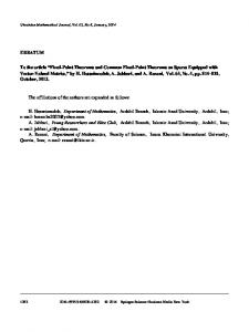
Case I. For x, y ∈ [0, 1], we have q(Sx, Ty) = {|
x y x 4 x 3y x − | + | |} ≤ {| − | + | |}. 12 8 12 5 4 4 4
Unauthenticated Download Date | 12/1/17 3:57 AM
Common fixed point theorems in QPMS
| 285
2
1.5
1
0.5
O
common fixed point
0.5
1
1.5
2
Figure 1: Case-I, (2D-View).
In Figure 1: Case-I, (2D-view), the red line denotes Ax, the yellow line denotes Ty, the green line denotes Sx, the brown line denotes By, the black line denotes y = x, the blue line denotes the right hand-side of the function and the orange line denotes the left hand-side of the function. Clearly, the functions A, B, S and T intersect on the line y = x only at x = 0, i.e., x = 0 is the unique common fixed point of A, B, S and T.
–
0.4
0.2 common fixed point
1
O
0 0
0.2
0.5 0.4
0.6
0.8
10
Figure 2: Case-I, (3D-view).
–
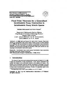
In Figure 2: Case-I, (3D-view), the plane in blue colour denotes the left hand-side of the inequality and the plane in red colour denotes the right hand-side of the inequality. Clearly, the figure verifies that the left handside with the blue surface is dominated by the right hand-side with the red surface. Hence, the inequality (3.2) is satisfied for x, y ∈ [0, 1].
Case II. For x ∈ [0, 1] and y ∈ (1, 2], we have q(Sx, Ty) = {|
x 1 x 4 3 1 3 − | + | |} ≤ {| − | + | |}. 12 8 12 5 4 8 4
Unauthenticated Download Date | 12/1/17 3:57 AM
286 | Anita Tomar, Said Beloul, Ritu Sharma, and Shivangi Upadhyay 2
1.5
1
0.5
0.5
1
1.5
2
Figure 3: Case-II, (2D-View).
–
In Figure 3: Case-II, (2D-view), the red line denotes Ax, the yellow line denotes Ty, the green line denotes Sx, the brown line denotes By and the black line denotes y = x.
1
0.5 2 0
0.2
1.5 0.4
0.6
0.8
11
Figure 4: Case-II, (3D-view).
–
In Figure 4: Case-II, (3D-view), the plane in blue colour denotes the left hand-side of the inequality and the plane in red colour denotes the right hand-side of the inequality. Clearly, the figure verifies that the left handside with the blue surface is dominated by the right hand-side with the red surface. Hence, the inequality (3.2) is satisfied for x ∈ [0, 1] and y ∈ (1, 2].
Case III. For x ∈ (1, 2] and y ∈ [0, 1], we have q(Sx, Ty) = {|
1 y 1 4 5 3y 5 − | + | |} ≤ {| − | + | |}. 4 8 4 5 8 4 8
Unauthenticated Download Date | 12/1/17 3:57 AM
Common fixed point theorems in QPMS
| 287
2
1.5
1
0.5
0.5
1
1.5
2
Figure 5: Case-III, (2D-View).
–
In Figure 5: Case-III, (2D-view), the red line denotes Ax, the brown line denotes Ty, the green line denotes Sx, the yellow line denotes By and the black line denotes y = x.
4
2 1 0 1
1.2
0.5 1.4
1.6
1.8
20
Figure 6: Case-III, (3D-View).
–
In Figure 6: Case-III, (3D-view), the plane with blue surface denotes the left hand-side of the inequality and the plane with red surface denotes the right hand-side of the inequality. Clearly, the figure verifies that the left hand-side with the blue surface is dominated by the right hand-side with the red surface. Hence, the inequality (3.2) is satisfied for x ∈ (1, 2] and y ∈ [0, 1].
Case IV. For x, y ∈ (1, 2], we have q(Sx, Ty) = {|
1 1 1 4 3 1 3 − | + | |} ≤ {| − | + | |}. 4 8 4 5 4 8 4
Unauthenticated Download Date | 12/1/17 3:57 AM
288 | Anita Tomar, Said Beloul, Ritu Sharma, and Shivangi Upadhyay 2
1.5
1
0.5
0.5
1
1.5
2
Figure 7: Case-IV, (2D-view).
–
In Figure 7: Case-IV, (2D-view), the red line denotes Ax, the brown line denotes Ty, the green line denotes Sx, the yellow line denotes By and the black line denotes y = x.
1
2
0.5 1
1.2
1.5 1.4
1.6
1.8
21
Figure 8: Case-IV, (3D-view).
–
In Figure 8: Case-IV, (3D-view), the plane with blue surface denotes the left hand-side of the inequality and the plane with red surface denotes the right hand-side of the inequality. Clearly, the figure verifies that the left hand-side with blue surface is dominated by the right hand-side with the red surface. Hence, the inequality (3.2) is satisfied for x and y ∈ (1, 2].
Consequently, all hypotheses of Theorem 3.1 are satisfied (for δ = fixed point of A, B, S and T.
4 5
and L = 0) and 0 is the unique common
If A = B and S = T, we get the following Corollary Corollary 3.1. Let A and T be self mappings of a quasi-partial metric space (X, q). If A satisfies generalized condition (B) associated with T for all x, y ∈ X and we have
Unauthenticated Download Date | 12/1/17 3:57 AM
Common fixed point theorems in QPMS
1. 2. 3.
| 289
TX ⊂ AX, AX is closed, (δ + 2L) < 1,
then A and T have a coincidence point. Further, A and T have a unique common fixed point, provided that the pair (A, T) is weakly compatible. It is worth mentioning here that Corollary 3.1 extends Theorem 2.1, Theorem 2.2 and Corollary 2.3 in [4] in the setting of a quasi-partial metric space. Corollary 3.2. Let A, B, S and T be self mappings of a quasi-partial metric space (X, q). If the pairs of mappings (A, S) and (B, T) satisfy q(Sx, Ty) ≤ δ max{q(Ax, By), q(Ax, Sx), q(By, Ty),
1 (q(Sx, By) + q(Ax, Ty))} 2
for all x, y ∈ X and we have 1. TX ⊂ AX and SX ⊂ BX, 2. AX or BX is closed, then the pairs (A, S) and (B, T) have a coincidence point. Further, A, B, S and T have a unique common fixed point, provided that the pairs (A, S) and (B, T) are weakly compatible. Proof. The Proof follows similar lines to the proof of Theorem 3.1, using L = 0. Corollary 3.3. Let A and T be self mappings of a quasi-partial metric space (X, q). If the pair of mappings (A, T) satisfies q(Tx, Ty) ≤ δ max{q(Ax, Ay), q(Ax, Tx), q(Ay, Ty),
1 (q(Tx, Ay) + q(Ax, Ty))} 2
for all x, y ∈ X and we have 1. TX ⊂ AX, 2. AX is closed, then the pair (A, T) has a coincidence point. Further, A and T have a unique common fixed point, provided that the pair (A, T) is weakly compatible. Proof. The Proof follows similar lines to the proof of Theorem 3.1, using L = 0, A = B and S = T. Corollary 3.4. Let A and T be self mappings of a quasi-partial metric space (X, q). If the pair of mappings (A, T) satisfies q(Tx, Ty) ≤ δq(Ax, Ay) for all x, y ∈ X and we have 1. TX ⊂ AX, 2. AX is closed, then the pair (A, T) has a coincidence point. Further, A and T have a unique common fixed point, provided that the pair (A, T) is weakly compatible. Proof. The Proof follows similar lines to the proof of Theorem 3.1. The result is slightly more interesting when the closure of the range space TX or SX is considered.
Unauthenticated Download Date | 12/1/17 3:57 AM
290 | Anita Tomar, Said Beloul, Ritu Sharma, and Shivangi Upadhyay Theorem 3.2. Let A, B, S and T be self mappings of a quasi-partial metric space (X, q). If there exist δ ∈ (0, 1) and L ≥ 0, such that for all x, y ∈ X, the pairs of mappings (A, S) and (B, T) satisfy q(Sx, Ty) ≤ δ max{q(Ax, By), q(Ax, Sx), q(By, Ty), q(Ax, Ty), q(Sx, By)} + L min{q(Ax, Sx), q(By, Ty), q(Ax, Ty), q(By, Sx)}
(3.3)
and we have 1. TX ⊂ AX or SX ⊂ BX, 2. (δ + 2L) < 1, then the pairs (A, S) and (B, T) have a coincidence point. Further, A, B, S and T have a unique common fixed point, provided that the pairs (A, S) and (B, T) are weakly compatible. Proof. It can be proved following similar arguments to those given in the proof of Theorem 3.1. Example 3.3. Let X = [0, ∞) be endowed with the quasi-partial metric : q(x, y) = |x − y| + |x| and let A, B, S and T be mappings defined by ( ( x x, 0 ≤ x ≤ 1 2, 0 ≤ x ≤ 1 Ax = Bx = 2, x > 1, 1, x > 1, ( Sx =
x 10 ,
1,
Here we have TX = [0,
0≤x≤1 x > 1,
( Tx =
x 5, 1 2,
0≤x≤1 x > 1.
1 1 ] ∪ { } ⊂ [0, 1] ∪ {2} = AX, 5 2
1 1 ] ∪ {1} ⊂ [0, ] ∪ {1} = BX. 10 2 The point 0 is a coincidence point of the four mappings. Further, AS0 = SA0 = 0 and TB0 = BT0 = 0, i.e., both the pairs (A, S) and (B, T) are weakly compatible. SX = [0,
Case I. For x, y ∈ [0, 1], we have q(Sx, Ty) = |
x y x 1 5 y − |+| |= {| 2x − y | + | x |} ≤ {| x − | + | x |}. 10 5 10 10 9 2
3
2
1
O
common fixed point
0.5
1
1.5
2
2.5
3
Figure 9: Case-I, (2D-view).
Unauthenticated Download Date | 12/1/17 3:57 AM
Common fixed point theorems in QPMS |
291
In Figure 9: In Case-I, (2D-view), the red line denotes Ax, the yellow line denotes Ty, the green line denotes Sx, the brown line denotes By, the pink line denotes the right hand-side of the function, the orange line denotes the left hand-side of the function and the black line denotes y = x. Clearly, the functions A, B, S and T intersect on the line y = x only at x = 0, i.e., x = 0 is the unique common fixed point of A, B, S and T.
–
0.4
0.2 common fixed point
1
O
0 0
0.2
0.5 0.4
0.6
0.8
10
Figure 10: Case-I, (3D-view).
In Figure 10: Case-I, (3D-view), the plane in blue colour denotes the left hand-side of the inequality and the plane in red colour denotes the right hand-side of the inequality. Clearly, the figure verifies that the left handside with the blue surface is dominated by the right hand-side with the red surface. Hence, the inequality (3.3) is satisfied for x, y ∈ [0, 1].
–
Case II. For x ∈ [0, 1] and y > 1, we have q(Sx, Ty) = |
x 1 x 5 1 − | + | | ≤ {|1 − | + |1|}. 10 2 10 9 2
3
2
1
O
0.5
1
1.5
2
2.5
3
Figure 11: Case-II, (2D-view).
Unauthenticated Download Date | 12/1/17 3:57 AM
292 | Anita Tomar, Said Beloul, Ritu Sharma, and Shivangi Upadhyay In Figure 11: In Case-II, (2D-view), the red line denotes Ax, the yellow line denotes Ty, the green line denotes Sx, the brown line denotes By and the black line denotes y = x.
–
0.8
0.6
0
2 0.2
1.5 0.4
0.6
0.8
11
Figure 12: Case-II, (3D-view).
In Figure 12: Case-II, (3D-view), the plane in blue colour denotes the left hand-side of the inequality and the plane in red colour denotes the right hand-side of the inequality. Clearly, the figure verifies that the left handside with the blue surface is dominated by the right hand-side with the red surface. Hence, the inequality (3.3) is satisfied for x ∈ [0, 1] and y > 1.
–
O
Case III. For x > 1 and y ∈ [0, 1], we have q(Sx, Ty) = |1 −
y 5 y | + |1| ≤ {|2 − | + |2|}. 5 9 5
3
2
1
0.5
1
1.5
2
2.5
3
Figure 13: Case-III, (2D-view).
–
In Figure 13: Case-III, (2D-view), the red line denotes Ax, the brown line denotes Ty, the green line denotes Sx, the yellow line denotes By and the black line denotes y = x.
Unauthenticated Download Date | 12/1/17 3:57 AM
Common fixed point theorems in QPMS |
293
4
3
2 1
1 1.2
0.5 1.4
1.6
1.8
20
Figure 14: Case-III, (3D-view).
In Figure 14: Case-III, (3D-view), the plane with the blue surface denotes the left hand-side of the inequality and the plane with the red surface denotes the right hand-side of the inequality. Clearly, the figure verifies that the left hand-side with the blue surface is dominated by the right hand-side with the red surface. Hence, the inequality (3.3) is satisfied for x > 1 and y ∈ [0, 1].
–
Case IV. For x, y > 1, we have q(Sx, Ty) = |1 −
1 15 | + |1| ≤ . 2 9
3
2
1
0.5
1
1.5
2
2.5
3
Figure 15: Case-IV, (2D-View).
–
In Figure 15: Case-IV, (2D-view), the red line denotes Ax, the brown line denotes Ty, the green line denotes Sx, the yellow line denotes By and the black line denotes y = x.
Unauthenticated Download Date | 12/1/17 3:57 AM
294 | Anita Tomar, Said Beloul, Ritu Sharma, and Shivangi Upadhyay
1.5 1 2
0.5 1
1.2
1.5 1.4
1.6
1.8
21
Figure 16: Case-IV, (3D-view).
–
In Figure 16: Case-IV, (3D-view), the plane with the blue surface denotes the left hand-side of the inequality and the plane with the red surface denotes the right hand-side of the inequality. Clearly, the figure verifies that the left hand-side with the blue surface is dominated by the right hand-side with the red surface. Hence, the inequality (3.3) is satisfied for x, y > 1.
Consequently, all hypotheses of Theorem 3.2 are satisfied (for δ = fixed point of A, B, S and T.
5 9
and L = 0) and 0 is the unique common
For A = B and S = T Theorem 3.2 reduces to following Corollary Corollary 3.5. Let A and T be self mappings of a quasi-partial metric space (X, q). If there exist δ ∈ (0, 1) and L ≥ 0, such that for all x, y ∈ X, the pair of mappings (A, T) satisfies q(Tx, Ty) ≤ max{q(Ax, Ay), q(Ax, Tx), q(Ay, Ty), q(Ax, Ty), q(Tx, Ay)} + L min{q(Ax, Tx), q(Ay, Ty), q(Ax, Ty), q(Ay, Tx)} and we have 1. TX ⊆ AX, 2. (δ + 2L) < 1, then the pair (A, T) has a coincidence point. Further, A and T have a unique common fixed point, provided that the pair (A, T) is weakly compatible. Abbas et al. [4] posed two open problems: Open problem 1. Is Theorem 3.1 [4] valid for 12 ≤ δ < 1? We answer affirmatively in the case of a non-complete quasi-partial metric space, assuming the closures of the range space TX or SX (TX ⊂ AX or SX ⊂ BX) and the pairs (A, S) and (B, T) to be weakly compatible. Hence, our Theorem 3.2 extends the results of Berinde [7] to two pairs of self mappings. It is also demonstrated by illustrative Example 3.2 that Theorem 3.2 is valid for δ = 59 . Open problem 2. Under what additional assumptions either on f and T, or on the domain of f and T, do the mappings f and T have common fixed points? In a non-complete quasi partial-metric space when the closure of the range space TX is considered (TX ⊂ fX),
Unauthenticated Download Date | 12/1/17 3:57 AM
Common fixed point theorems in QPMS |
295
the weakly compatible pair (f , T) of self mappings has a unique common fixed point (taking f = A in Corollary 3.5). Remark 3.1. We have established common fixed point theorems for quadruple of self mappings in a noncomplete quasi-partial metric space (X, q), satisfying generalized condition (B), without exploiting the notion of continuity or any of its variants like reciprocal continuity, weak reciprocal continuity, sub-sequential continuity, sequential continuity of type (Af ) or (Ag), conditional reciprocal continuity and so on. For details on variants of continuity one may refer to Tomar and Karapinar [17]. Remark 3.2. Since (X, q) is not a metric space, generalized condition (B) for quadruple of self mappings does not reduce to any metric condition. Hence, our results do not reduce to the existing fixed point theorems in metric spaces. Our results generalize, extend and improve the results of Abbas [4], Abbas et al. [5], Babu et ` c [16], Kannan [14], Zamfirescu [15] and so on to quasial. [6], Banach [13], Berinde [7], Chatterjea [8], Ciri` partial metric spaces. A more natural condition of closedness of the range space is assumed to establish a unique common fixed point.
4 Application To Integral Equations Consider the following integral equation ZL K(l, s, u(s))ds + g(l),
u(l) =
(4.1)
0
where l ∈ [0, L], L > 0, K : [0, L] × [0, L] × R → R and g : R → R. The aim of this section is to give an existence theorem for a solution to the above integral equation using Corollary 3.4. Let X = [0, L]. Define q : X × X → R+ by q(x, y) = sup l∈[0,L] |x(l) − y(l)| + sup l∈[0,L] |x(l)|. Then (X, q) is a quasi-partial metric space. Theorem 4.1. Let T, A : [0, L] → [0, L] be self mappings of a quasi-partial metric space (X, q). Suppose the following hypotheses hold: (H1 ) : ZL Tx(l) = K1 (l, s, x(s))ds + g(l), l ∈ [0, L], 0
and
ZL Ax(l) =
K2 (l, s, x(s))ds + g(l), l ∈ [0, L], 0
where K1 , K2 : [0, L] × [0, L] × R → R, (H2 ) :|K1 (l, s, u(l)) − K1 (l, s, v(l)| ≤ h(l, s){|Au − Av| + |Au|} for each u, v ∈ R and each l, s ∈ [0, L], ZL (H3 ) : sup h(l, s)ds ≤ δ for some δ ∈ [0, 1), l∈[0,L]
0
(H4 ) :TX ⊂ AX and AX is closed, (H5 ) :ATx = TAx, whenever Ax = Tx for some x ∈ [0, L].
Unauthenticated Download Date | 12/1/17 3:57 AM
296 | Anita Tomar, Said Beloul, Ritu Sharma, and Shivangi Upadhyay Then the integral equation (4.1) has a unique solution u ∈ [0, L]. Proof. Clearly TX ⊂ AX and AX is closed. Now, we have q(Tx, Ty) = sup l∈[0,L] |Tx(l) − Ty(l)| + sup l∈[0,L] |Tx(l)| ZL
ZL K1 (l, s, x(s))ds −
=| 0
ZL K1 (l, s, y(s))ds| + |
0
0
ZL
ZL
|K1 (l, s, x(s))|ds
|K1 (l, s, x(s)) − K1 (l, s, y(s))|ds +
≤
K1 (l, s, x(s))ds|
0
0
ZL ≤ (sup l∈[0,L] |Ax(s) − Ay(s)| + sup l∈[0,L] |Ax(s)|)sup l∈[0,L]
h(l, s)ds 0
ZL = q(Ax, Ay)sup l∈[0,L]
h(l, s)ds. 0
By hypothesis (H3 ), there exists δ ∈ [0, 1), such that ZL sup l∈[0,L]
h(l, s)ds < δ. 0
Thus, we have q(Tx, Ty) ≤ δq(Ax, Ay). Hence, all the hypotheses of Corollary 3.4 are satisfied and there exists a unique common fixed point u ∈ [0, L] of A and T, i.e., there exists a unique solution u ∈ X to the integral equation (4.1).
5 Application To Functional Equations Arising In Dynamic Programming Problem The existence and uniqueness of solutions to functional equations arising in dynamic programming have been studied by various authors (see [18, 19] and references therein). In this section we prove existence and uniqueness of a solution for a class of functional equations in a quasi-partial metric space using Corollary 3.4. Let U and V be Banach spaces, W ⊂ U is a state space, D ⊂ V is a decision space and R is the field of real numbers. Let X = B(W) denote the set of all closed and bounded real valued functions on W . Consider the following functional equation p(x) = sup y∈D {g(x, y) + M(x, y, p(τ(x, y)))}, x ∈ W .
(5.1)
Let g : W × D → R and M : W × D × R → R be bounded functions. τ : W × D → W represents transformation of the process and p(x) represents the optimal return function with initial state x. For an arbitrary h ∈ B(W) define khk = sup |h(x)|. Also, (B(W), k.k) is a Banach space wherein convergence is uniform. Define q : X × X → R+ by q(x, y) = |x − y| + |x|, then (X, q) is a quasi-partial metric space. Theorem 5.1. Let T, A : B(W) → B(W) be self mappings of a quasi-partial metric space (B(W), q). Suppose there exists a δ ∈ [0, 1) such that for every (x, y) ∈ W × D, Ah1 , Ah2 ∈ B(W) and t ∈ W :
Unauthenticated Download Date | 12/1/17 3:57 AM
Common fixed point theorems in QPMS |
1. 2. 3.
297
|M(x, y, Ah1 τ(x, y)) − M(x, y, Ah2 τ(x, y))| ≤ δ{|Ah1 τ(x, y) − Ah2 τ(x, y)| + |Ah1 τ(x, y)|} holds; g : W × D → R and M : W × D × R → R are bounded functions; ATh = TAh, whenever Ah = Th, for some h ∈ B(W).
Then the functional equation Th i (x) = sup{g(x, y) + M(x, y, Ah i (τ(x, y)))}, x, y ∈ W
(5.2)
y∈D
has a unique bounded solution in B(W). Proof. By hypothesis (3), the pair (A, T) is weakly compatible. Let λ be an arbitrary positive real number and Ah1 , Ah2 ∈ B(W). For x ∈ W , we choose y1 , y2 ∈ D so that T(h1 (x)) < g(x, y1 ) + M(x, y1 , Ah1 (τ1 )) + λ,
(5.3)
T(h2 (x)) < g(x, y2 ) + M(x, y2 , Ah2 (τ2 )) + λ,
(5.4)
where τ1 = τ(x, y1 ) and τ2 = τ(x, y2 ). From the definition of the mapping T, we have T(h1 (x)) ≥ g(x, y2 ) + M(x, y2 , Ah1 (τ2 )),
(5.5)
T(h2 (x)) ≥ g(x, y1 ) + M(x, y1 , Ah2 (τ1 )).
(5.6)
Now, from (5.3) and (5.6), we obtain T(h1 (x)) − T(h2 (x)) < M(x, y1 , Ah1 (τ1 )) − M(x, y1 , Ah2 (τ1 )) + λ ≤ |M(x, y1 , Ah1 (τ1 )) − M(x, y1 , Ah2 (τ1 ))| + λ ≤ δ{|Ah1 − Ah2 | + |Ah1 |} + λ. Similarly, from (5.4) and (5.5), we obtain T(h2 (x)) − T(h1 (x)) ≤ δ{|Ah1 − Ah2 | + |Ah1 |} + λ Hence, we have |T(h1 (x)) − T(h2 (x))| ≤ δ{|Ah1 − Ah2 | + |Ah1 |} + λ.
(5.7)
Since the inequality (5.7) is true for all x ∈ W and arbitrary λ > 0, then we have q(Th1 , Th2 ) ≤ δq(Ah1 , Ah2 ). Thus, all the conditions of Corollary 3.4 are satisfied and hence the mappings, A and T have a unique common fixed point, i.e., the functional equation (5.2) has a unique bounded solution.
6 Conclusion Generalized condition (B) is introduced in a quasi-partial metric space to establish coincidence and common fixed point for two weakly compatible pairs of self-mappings using more natural condition of closedness of the range space. Results are validated with the help of explanatory examples associated with pictographic validations. The motivation behind using a partial quasi-metric space is the fact that the distance from point x to point y may be different to that from y to x and the self-distance of a point need not always be zero. It
Unauthenticated Download Date | 12/1/17 3:57 AM
298 | Anita Tomar, Said Beloul, Ritu Sharma, and Shivangi Upadhyay is interesting to see that although several authors claimed to have introduced some weaker notions of commuting mappings, weak compatibility is still the minimal and the most widely used notion among all weaker variants of commutativity. For brief development of weaker forms of commuting mappings one may refer to Singh and Tomar [20]. Further results obtained are utilised to establish the existence and uniqueness of a solution to the integral equation and the functional equation arising in dynamic programming. Acknowledgement: The authors are grateful to the knowledgeable referee for his careful reading of the manuscript and for giving valuable remarks and suggestions to improve this paper.
References [1] [2] [3] [4] [5] [6] [7] [8] [9] [10] [11] [12] [13] [14] [15] [16] [17] [18] [19] [20]
Fr`echet M., Sur quelques points du calcul fonctionnel, Rendic. Circ. Mat. Palermo, 1906, 22, 1-74 K¨ unzi H.-P. A., Pajoohesh H., Schellekens M. P., Partial quasi-metrics, Theoret. Comput. Sci., 2006, 365(3), 237-246 ¨ urk Ali, Fixed point theorems on quasi-partial metric spaces, Math. Comput. Modelling, 2013, 57, Karapinar E., Erhan M., Ozt¨ 2442-2448 Abbas M., Babu G. V. R., Alemayehu G. N., On common fixed points of weakly compatible mappings satisfying generalized condition (B), Filomat, 2011, 25(2), 9-19 Abbas M., Nazir T., Vetro P., Common fixed point results for three maps in G-metric spaces, Filomat, 2011, 25(4), 1-17 Babu G. V. R., Sandhy M. L., Kameshwari M. V. R., A note on a fixed point theorem of Berinde on weak contractions, Carpathian J. Math. , 2008, 24(1), 8-12 ` c-type almost contractions in metric spaces, Carpathian J. Berinde V., General constructive fixed point theorems for Ciri` Math., 2008, 24(2), 10-19 Chatterjea S. K., Fixed point theorems, C. R. Acad. Bulgare Sci., 1972, 25, 727-730 Jungck G., Rhoades B. E., Fixed point for set valued functions without continuity, Indian J. Pure Appl. Math., 1998, 29(3), 227-238 Matthews S. G., Partial metric topology, Proceedings of the 8th Summer Conference on General Topology and Applications, Ann. New York Acad. Sci., 1994, 728, 183-197 Matthews S. G., Partial metric topology, Research Report 212, Department of Computer Science, University of Warwick, 1992 Abbas M., Ilic D., Common fixed points of generalized almost nonexpansive mappings, Filomat, 2010, 24(3), 11-18 Banach S., Sur les opérations dans les ensembles abstraits et leur application aux l’équations intégrales Fund. Math., 1922, 3, 133-181 Kannan R., Some results on fixed points, Bull.Calcutta Math. Soc., 1968, 60, 71-76 Zamfirescu T., Fixed point theorems in metric spaces, Arch. Math. (Basel), 1972, 23, 292-298 ` c L.B., A generalization of Banach principle, Proc. Amer. Math. Soc., 1974, 45, 727-730 Ciri` Tomar A., Karapinar E., On variants of continuity and existence of fixed point via Meir-Keeler contractions in MC-spaces, J. Adv. Math. Stud., 2016, 9(2), 348-359 Singh S. L., Mishra S. N., Remarks on recent fixed point theorems, Fixed Point Theory Appl., 2010, Article ID 452905, 18 pages Singh S. L., Mishra S. N., Coincidence theorems for certain classes of hybrid contractions, Fixed Point Theory Appl., 2010, Article ID 898109, 14 pages Singh S. L., Tomar A., Weaker forms of commuting maps and existence of fixed points, J. Korea Soc. Math. Educ. Ser. B Pure Appl. Math., 2003, 10(3), 141-161
Unauthenticated Download Date | 12/1/17 3:57 AM