Communities Validity: Methodical Evaluation of Community Mining

Noname manuscript No. (will be inserted by the editor)

Communities Validity: Methodical Evaluation of Community Mining Algorithms Reihaneh Rabbany · Mansoureh Takaffoli · Justin Fagnan · Osmar R. Za¨ıane · Ricardo J. G. B. Campello

the date of receipt and acceptance should be inserted later

Abstract Grouping data points is one of the fundamental tasks in data mining, which is commonly known as clustering if data points are described by attributes. When dealing with interrelated data that is represented in the form of nodes and their relationships and the grouping is based on these relationships but not the node attributes, this task is also referred to as community mining. There has been a considerable number of approaches proposed in recent years for mining communities in a given network. However, little work has been done on how to evaluate the community mining algorithms. The common practice is to evaluate the algorithms based on their performance on standard benchmarks for which we know the ground-truth. This technique is similar to external evaluation of attribute-based clustering methods. The other two well-studied clustering evaluation approaches are less explored in the community mining context; internal evaluation to statistically validate the clustering result, and relative evaluation to compare alternative clustering results. These two approaches enable us to validate communities discovered in a real world application, where the true community structure is hidden in the data. In this article, we investigate different clustering quality criteria applied for relative and internal evaluation of clustering data points with attributes, and also different clustering agreement measures used for external evaluation; and incorporate proper adaptations to make them applicable in the context of interrelated data. We further compare the performance of the proposed adapted criteria in evaluating community mining results in different settings through extensive set of experiments. Keywords Evaluation Approaches · Quality Measures · Clustering Evaluation · Clustering Objective Function · Community Mining Reihaneh Rabbany · Mansoureh Takaffoli · Justin Fagnan · Osmar R. Za¨ıane · Ricardo J. G. B. Campello Department of Computing Science, University of Alberta, Edmonton, Canada Tel.: +1-780-492-{3978,2860}, Fax: +1-780-492-1071 E-mail: {rabbanyk, takaffol, fagnan, zaiane, rcampell}@ualberta.ca

2

Rabbany et al.

1 Introduction Data Mining is the analysis of large scale data to discover meaningful patterns such as groups of data records (cluster analysis), unusual records (anomaly detection) or dependencies (association rule mining) which are crucial in a very broad range of applications. It is a multidisciplinary field that involves methods at the intersection of artificial intelligence, machine learning, statistics and database systems. The recent growing trend in the Data Mining field is the analysis of structured/interrelated data, motivated by the natural presence of relationships between data points in a variety of the present-day applications. The structures in these interrelated data are typically modeled by a graph of interconnected nodes, known as complex networks or information networks. Examples of such networks are hyperlink networks of web pages, citation or collaboration networks of scholars, biological networks of genes or proteins, trust and social networks of humans among others. All these networks exhibit common statistical properties, such as power law degree distribution, small-world phenomenon, relatively high transitivity, shrinking diameter, and densification power laws. Network clustering, a.k.a. community mining, is one of the principal tasks in the analysis of complex networks. Many community mining algorithms have been proposed in recent years: for surveys refer to Fortunato (2010), Porter et al. (2009). These algorithms evolved very quickly from simple heuristic approaches to more sophisticated optimization based methods that are explicitly or implicitly trying to maximize the goodness of the discovered communities. The broadly used explicit maximization objective is the modularity introduced by Newman and Girvan (2004). Although there have been many methods proposed for community mining, very little research has been done to explore evaluation and validation methodologies. Similar to the well-studied clustering validity methods in the Machine Learning field, we have three classes of approaches to evaluate community mining algorithms; external, internal and relative evaluation. The first two are statistical tests that measure the degree to which a clustering confirms a-priori specified scheme. The third approach compares and ranks clusterings of a same dataset discovered by different parameter settings (Halkidi et al. 2001). In this article, we investigate the evaluation approaches of community mining algorithms, considering this same classification. External evaluation involves comparing the discovered clustering with a prespecified structure, often called ground-truth, using a clustering agreement measure such as Jaccard, Adjusted Rand Index, or Normalized Mutual Information. In the case of attribute-based data, clustering similarity measures are not only used for evaluation, but also applied to determine the number of clusters in a data set, or to combine different clustering results and obtain a consensus clustering i.e. ensemble clustering (Vinh et al. 2010). In the interrelated data context, these measures are used commonly for external evaluation of community mining algorithms, where the performance of the algorithms are examined on standard benchmarks for which we know the true communities

Communities Validity

3

(Chen et al. 2009b, Danon et al. 2005, Lancichinetti and Fortunato 2009, Orman et al. 2011). In Section 3.2 of this article, we overview the well-known clustering agreement measures and elaborate on the considerations of using them for community mining evaluation. There are few and typically small real world benchmarks with known communities available for external evaluaion of community mining algorithms, while the current synthetic benchmark generators used for generating benchmarks with built-in ground-truth, overlook some characteristics of the real networks (Orman and Labatut 2010). Moreover, in a real-world application, the interesting communities that need to be discovered are hidden in the structure of the network, thus, the discovered communities can not be validated based on the external evaluation. These facts motivate investigating the other two alternatives approaches – internal and relative evaluation. Internal evaluation techniques verify whether the clustering structure produced by a clustering algorithm matches the underlying structure of the data, using only information inherent in the data. These techniques are based on an internal criterion that measures the correlation between the structure of the data, represented as a proximity matrix1 , and the discovered clustering structure. The significance of this correlation is examined statistically based on the distribution of the defined criteira, which is usually not known and is estimated using Monte Carlo sampling method (Theodoridis and Koutroumbas 2009). An internal criterion can also be considered as a quality index to compare different clusterings which overlaps with relative evaluation techniques. The well-known modularity of Newman (2006) can be considered as such, which is used both to validate a single community mining result and also to compare different community mining results (Clauset 2005, Rosvall and Bergstrom 2007). Modularity is defined as the fraction of edges within communities, i.e. the correlation of adjecency matrix and the clustering structure, minus the expected value of this fraction that is computed based on the configuration model (Newman 2006). Relative evaluation compares alternative clustering structures based on an objective function or quality index. This evaluation approach is the least explored in the community mining context. Defining an objective function to evaluate community mining is non-trivial. Aside from the subjective nature of the community mining task, there is no formal definition on the term community. Consequently, there is no consensus on how to measure “goodness” of the discovered communities by a mining algorithm. Nevertheless, the well-studied clustering methods in the Machine Learning field are subject to similar issues and yet there exists an extensive set of validity criteria defined for clustering evaluation, such as Davies-Bouldin index (Davies and Bouldin 1979), Dunn index (Dunn 1974), and Silhouette (Rousseeuw 1987); for a recent survey refer to Vendramin et al. (2010). In Section 3.1 of this article, we describe how these criteria could be adapted to the context of community mining in order to 1 A square matrix in which the entry in cell (j, k) is some measure of the similarity (or distance) between the items i, and j.

4

Rabbany et al.

compare results of different community mining algorithms. Also, these criteria can be used as alternatives to modularity to design novel community mining algorithms. In the following, we first briefly introduce well-known community mining algorithms, and common evaluation practices including available benchmarks. Next, we overview the clustering validity criteria and clustering similarity measures and propose proper adaptions these measures require to handle comparison of community mining results. Then, we extensively compare and discuss the adapted criteria on real and synthetic networks. Finally, we conclude with a brief analysis of these results.

2 Related Work A community is roughly defined as “densely connected” individuals that are “loosely connected” to others outside their group. A great number of community mining algorithms have been developed in the last few years having different interpretations of this definition. Basic heuristic approaches mine communities by assuming that the network of interest divides naturally into some subgroups, determined by the network itself. For instance, the Clique Percolation Method (Palla et al. 2005) finds groups of nodes that can be reached via chains of k-cliques. The common optimization approaches mine communities by maximizing the overall “goodness” of the result. The most credible “goodness” objective is known as modularity Q, proposed in (Newman and Girvan 2004), which considers the difference between the fraction of edges that are within the communities and the expected such fraction if the edges are randomly distributed. Several community mining algorithms for optimizing the modularity Q have been proposed, such as fast modularity (Newman 2006), and Max-Min modularity (Chen et al. 2009b). Furthermore, for large networks in which the global information is not available or computationaly expensive, local community mining algorithms based on local versions of this measure are developed. Local modularity M (Luo et al. 2008), and local modularity L (Chen et al. 2009a), are local variants of modularity Q, where the ratio of internal and external edges is calculated by identifying boundary nodes of a detected local community. Although many mining algorithms are based on the concept of modularity, Fortunato and Barth´elemy (2007) have shown that the modularity cannot accurately evaluate small communities due to its resolution limit. Hence, any algorithm based on modularity is biased against small communities. As an alternative to optimizing modularity Q, we previously proposed TopLeaders community mining approach (Rabbany et al. 2010), which implicitly maximizes the overall closeness of followers and leaders, assuming that a community is a set of followers congregating around a potential leader. There are many other alternative methods. One notable family of approaches mine communities by utilizing information theory concepts such as compression e.g. Infomap (Rosvall and Bergstrom 2008), and entropy

Communities Validity

5

e.g. entropy-base (Kenley and Cho 2011). For a survey on different community mining techniques refer to (Fortunato 2010). Fortunato (2010) shows that the different community mining algorithms discover communities from different perspective and may outperform others in specific classes of networks and have different computational complexities. Therefore, an important research direction is to evaluate and compare the results of different community mining algorithms, and select the one providing more meaningful clustering for each class of networks. An intuitive practice is to validate the results partly by a human expert (Luo et al. 2008). However, the community mining problem is NP-complete; the human expert validation is limited and based on narrow intuition rather than on an exhaustive examination of the relations in the given network, specially for large real networks. To validate the result of a community mining algorithm, three approaches are available; external evaluation, internal evaluation, and relative evaluation. The external evaluation technique measures the degree of correspondence between the known and true clustering (i.e. ground-truth) of the underlying dataset and the clustering that results after applying a specific community mining algorithm to the dataset. To measure agreement between two clusterings, a clustering agreement measure should be used. Two main families of agreement measures are available: 1) pair counting approaches that rely on counting pairs of items on which two clusterings agree or disagree. (e.g. Jaccard); 2) information theoretic approaches that are based on measuring the information shared by two clusterings (e.g. Normalized Mutual Information (NMI)). The external evaluation requires knowing the true communities, however, for almost all real-world networks, the true communities are unknown and need to be discovered by the community mining algorithms. Therefore, to validate different community mining algorithms, we mainly apply external evaluation on two cases: 1) real benchmark datasets with known community structure; 2) synthetic networks with built-in ground-truth. In the literature, there are very few typically small real-world datasets that their true communities are known such as Karate Club by Zachary (Zachary 1977), Sawmill Strike data-set (Nooy et al. 2004), NCAA Football Bowl Subdivision (Girvan and Newman 2002), and Politician Books from Amazon (Krebs 2004). The standard procedure is to assess the agreement between the communities discovered by an algorithm and the true communities on these real dataset. To synthesize networks with built-in ground truth, several generators are proposed. GN benchmark (Girvan and Newman 2002) is the first synthetic network generator. This benchmark is a graph with 128 nodes, with expected degree of 16, and is divided into four groups of equal sizes; where the probabilities of the existence of a link between a pair of nodes of the same group and of different groups are zin and 1 − zin , respectively. However, the same expected degree for all the nodes, and equal-size communities are not accordant to real social network properties. LFR benchmark (Lancichinetti et al. 2008) amends GN benchmark by considering power law distributions for degrees and community sizes. Similar to GN benchmark, each node shares a fraction 1 − µ

6

Rabbany et al.

of its links with the other nodes of its community and a fraction µ with the other nodes of the network. However, having the same mixing parameter µ for all nodes, and not satisfying the densification power laws and heavy-tailed distribution are the main drawback of this benchmark. After generating synthetic networks with built-in community structure using any of the network generators, the accuracy of a community mining algorithm is then determined by comparing the discovered communities with the ground-truth. There are recent studies on the external evaluation of different community mining algorithms. Gustafsson et al. (2006) compare hierarchical and k-means community mining on real networks and also synthetic networks generated by the GN benchmark. Lancichinetti and Fortunato (2009) compare a total of a dozen community mining algorithms. The performance of the algorithms is compared against the network generated by both GN and LFR benchmark. Orman et al. (2011) compare a total of five community mining algorithms on the synthetic networks generated by LFR benchmark. They first assess the quality of the different algorithms by their difference with the ground truth. Then, they perform a qualitative analysis of the identified communities by comparing their size distribution with the community size distribution of the ground truth. However, none of the mentioned work focus on comparing different clustering agreement measures in the context of interrelated data. Thus, in this paper we overview different agreement measures existing in the literature, and also provide an alternative measure which works better on interrelated data. Internal evaluation is the second approach to validate different community mining algorithms. This technique validates the significance of correlation between the discovered community structure and the structural information inherent in the data. The structural information usually infers from proximity matrix (similarity or distance matrix), thus, a common practice here is to measure the correlation between the detected communities and the proximity matrix using Monte Carlo Sampling method. The internal evaluation of different community mining algorithms is studied in (Leskovec et al. 2010). They propose network community profile (NCP) that characterizes the quality of communities as a function of their size. The quality of the community at each size is characterized by the notion of conductance which is the ratio between the number of edges inside the community and the number of edges leaving the community. Then, they compared the shape of the NCP for different algorithms over random and real networks. The external and internal evaluation are both statistical approaches and require prior knowledge on the community structure or the properties inherent in the network. Relative evaluation, is a different approach that does not depend on prior knowledge. Here, a set of community mining algorithms is considered and the goal is to choose the best one according to a predefined objective function - criterion. In the context of interrelated data, up to now, mainly modularity Q is used as objective function to compare different community mining algorithms with each other (Rosvall and Bergstrom 2007). Therefore, in this article, we investigate other potential validity criteria for comparing

Communities Validity

7

different (non-overlapping) community mining results and examine the performance of these measures parallel to the modularity Q. In the future, these criteria not only can be used as a means to measure the goodness of discovered communities, but also as an objective function to detect communities.

3 Evaluation of Community Mining Results In this section, we elaborate on how to evaluate results of a community mining algorithm based on external and relative evaluation. External evaluation of community mining results involves comparing the discovered communities with a prespecified community structure, often called ground truth, using a clustering agreement measure, while the relative evaluation ranks different alternative community structures based on an objective function – quality index (Theodoridis and Koutroumbas 2009). To be consistent with the terms used in attribute-based data, we use clustering to refer to the result of any community mining algorithm, and partitioning to refer to the case where the communities are mutually exclusive. Note that, in this study we only focus on non-overlapping community mining algorithms that always produce disjoint communities. Thus, in the definition of the following quality criteria and agreement measures, partitioning is used instead of clustering which implies that the these are only applicable in the case of mutually exclusive communities. In the rest, we first overview relative community quality criteria, then describe different clustering agreement measures.

3.1 Community Quality Criteria Here, we overview several validity criteria that could be used as relative indexes for comparing and evaluating different partitionings of a given network. All of these criteria are generalized from well-known clustering criteria. The clustering quality criteria are originally defined with the implicit assumption that data points consist of vectors of attributes. Consequently their definition is mostly integrated or mixed with the definition of the distance measure between data points. The commonly used distance measure is the Euclidean distance, which cannot be defined for graphs. Therefore, we first review different possible proximity measures that could be used in graphs. Then, we present generalizations of criteria that could use any notion of proximity. 3.1.1 Proximity Between Nodes Let A denote the adjacency matrix of the graph, and let Aij be the weight of the edge between nodes ni and nj . The proximity between ni and nj , pij = p(i, j), can be computed by one of the following distance or similarity measures. The latter is more typical in the context of interrelated data, therefore, we tried to plug-in similarities in the relative criteria definitions. When

8

Rabbany et al.

it is not straightforward, we used the inverse of the similarity index to obtain the according dissimilarity/distance2 . Shortest Path (SP): distance between two nodes is the length of the shortest path between them, which could be computed using the well-known Dijkstra’s Shortest Path algorithm. Adjacency (A): similarity between the two nodes ni and nj is considered their incident edge weight, pA ij = Aij ; accordingly, the distance between these nodes is derived as: A dA ij = M − pij where M is the maximum edge weight in the graph; M = Amax = maxij Aij . Adjacency Relation (AR): distance between two nodes is their structural dissimilarity, that is computed by the difference between their immediate neighbourhoods (Wasserman and Faust 1994): sX (Aik − Ajk )2 dAR = ij k6=j,i

This definition is not affected by the (non)existence of an edge between the ˆ can be defined as; two nodes. To remedy this, Augmented AR (AR) sX ˆ = (Aˆik − Aˆjk )2 dAR ij k

where Aˆij is equal to Aij if i 6= j and Amax otherwise. Neighbour Overlap (NO): similarity between two nodes is the ratio of their shared neighbours (Fortunato 2010): O pN = |ℵi ∩ ℵj |/|ℵi ∪ ℵj | ij

where ℵi is the set of nodes directly connected to ni , ℵi = {nk |Aik 6= 0}. The O O corresponding distance is derived as dN = 1 − pN ij ij . There is a close relation between this measure and the previous one, since dAR can also be computed as: q dAR |ℵi ∪ ℵj | − |ℵi ∩ ℵj | ij = ˆ

while dAR ij is also derived from the same formula, if neighbourhoods are considered closed, i.e. ℵˆi = {nk |Aˆik 6= 0}. We also consider the closed neighbour ˆ overlap similarity, pN O , with the same analogy that two nodes are more similar ˆ if directly connected. The closed overlap similarity, pN O , could be rewritten 2 For avoiding division by zero, when P ij is zero, if it is a similarity  and if it is distance 1/ is returned, where  is a very small number, 10E-9.

Communities Validity

9

in terms of the adjacency matrix which can be straightforwardly generalized for weighted graphs. P ˆ ˆ k Aik Ajk 2 [Aˆ + Aˆ2 − Aˆik Aˆjk ]

ˆ

O pN =P ij

k

ˆ OV pN ij

ik

jk

P (Aˆik + Aˆjk )(Aˆik + Aˆjk ) − k (Aˆik − Aˆjk )(Aˆik − Aˆjk ) =P P ˆ (Aˆik + Aˆjk )(Aˆik + Aˆjk ) + (Aik − Aˆjk )(Aˆik − Aˆjk ) P

k

k

k

Topological Overlap (TP): similarity measures the normalized overlap size of the neighbourhoods (Ravasz et al. 2002), which we generalize as: (Aik Ajk ) + A2ij P 2 P 2 min( k Aik , k Ajk )

P pTijP

=

k6=j,i

and the corresponding distance is derived as dTijO = 1 − pTijO . Pearson Correlation (PC): coefficient between two nodes is the correlation between their corresponding rows of the adjacency matrix: P

C pP ij

=

k

(Aik − µi )(Ajk − µj ) N σi σj

P where N is p the number of nodes, the average µi = ( k Aik )/N and the variP 2 ance σi = k (Aik − µi ) /N . This correlation coefficient lies between −1 (when the two nodes are most similar) and 1 (when the two nodes are most dissimilar). Most relative clustering criteria are defined assuming distance is positive, therefore we also consider the normalized version of this correlation, C i.e. pN P C = (pP ij + 1)/2. Then, the distance between two nodes is computed (N )P C

(N )P C

as dij = 1 − pij . In all the above proximity measures, the iteration over all other nodes can be limited to iteration over the nodes in the P union of neighbourhoods. PN More specifically, in the formulas, one can use instead of k=1 . This k∈ℵˆi ∪ℵˆj will make the computation local and more efficient, especially in case of large networks. This trick will not work for the current definition of the pearson correlation, however, it can be applied if we reformulate it as follows: C pP ij

P

P P Aik Ajk − ( k Aik )( k Ajk )/N =q P P P P (( k A2ik ) − ( k Aik )2 /N )(( k A2jk ) − ( k Ajk )2 /N ) k

ˆ pPˆC , so that the existence of an We also consider this correlation based on A, edge between the two nodes, increases their correlation3 . 3

ˆ = N + 1 should be used. Note that since we are assuming a self edge for each node, N

10

Rabbany et al.

The above formula can be further rearranged as follows: i P h P P 2 0 0 A A − ( A )( A )/N 0 0 ik jk ik jk k k k C pP ij = r i P h i P h 2 P P ( k Aik − ( k0 Aik0 )2 /N 2 )( k A2jk − ( k0 Ajk0 )2 /N 2 ) Where if the k iterates over all nodes, it is equal to the original pearson correlation; P however, this is not true if it only iterates over the union of neighbourhoods, k∈ℵˆi ∪ℵˆj , which we call pearson overlap (N P O). Number of Paths (NP): between two nodes is the sum of all the paths between them, which is a notion of similarity. For the sake of time complexity, we consider paths of up to a certain number of hops i.e. 2 and 3. The number of paths of length l between nodes ni and nj can be computed as nplij = (Al )ij . More specifically we have: X X np1ij = Aij , np2ij = Aik Ajk , np3ij = Aik Akl Ajl k

kl NP 2

NP

3

where p is defined as a combination these; p = np1 + np2 and pN P = 1 2 3 np + np + np . We also considered two alternatives for this combination; p p 3 3 np3 np2 + , and pN PE = np1 + 2 np2 + 3 np3 pN PL = np1 + 2 3 Modularity (M): similarity is defined inspired by the Modularity of Newman (2006) as: P P ( k Aik )( k Ajk ) P pM = A − ij ij kl Akl A ij D P pM = P ij ( Aik )( Ajk ) k P k kl

The distance is derived as 1 − p

M (D)

Akl

.

ICloseness (IC): similarity between two nodes is computed as the inverse of the connectivity between their scored neighbourhoods: P ns(k, i)ns(k, j) pIC ij = P

k∈ℵi ∩ℵj

ns(k, i)2

k∈ℵi

+

P k∈ℵj

ns(k, j)2 −

P

ns(k, i)ns(k, j)

k∈ℵi ∩ℵj

a−b a+b X a= (ns(k, i) + ns(k, j))(ns(k, i) + ns(k, j))

pICV = ij

k∈ℵˆi ∪ℵˆj

b=

X k∈ℵˆi ∪ℵˆj

(ns(k, i) − ns(k, j))(ns(k, i) − ns(k, j))

Communities Validity

11

where ns(k, i) denotes the neighbouring score between nodes k and i that is computed iteratively; for complete formulation refer to (Rabbany and Za¨ıane 2011)4 . The distance is then derived as dIC(V ) = 1 − pIC(V ) . 3.1.2 Community Centroid In addition to the notion of proximity measure, most of the cluster validity criteria use averaging between the numerical data points to determine the centroid of a cluster. The averaging is not defined for nodes in a graph, therefore we modify the criteria definitions to use a generalized centroid notion, in a way that, if the centroid is set as averaging, we would obtain the original criteria definitions, but we could also use other alternative notions for centroid of a group of data points. Averaging data points results in a point with the least average distance to the other points. When averaging is not possible, using medoid is the natural option, which is perfectly compatible with graphs. More formally, the centroid of the community C can be obtained as the medoid: C = arg min m∈C

X

d(i, m)

i∈C

3.1.3 Relative Validity Criteria Here, we present our generalizations of well-known clustering validity criteria defined as quality measures for internal or relative evaluation of clustering results. All these criteria are originally defined based on distances between data points, which is in all cases the Euclidean or other inner product norms of difference between their vectors of attributes; refer to (Vendramin et al. 2010) for comparative analysis of these criteria in the clustering context. We alter the formulae to use a generalized distance, so that we can plug in our graph proximity measures. The other alteration is generalizing the mean over data points to a general centroid notion, which can be set as averaging in the presence of attributes and the medoid in our case of dealing with graphs and in the absence of attributes. In a nutshell, in every criterion, the average of points in a cluster is replaced with a generalized notion of centroid (Section 3.1.2), and distances between data points are generalized from Euclidean/norm to a generic distance (Section 3.1.1). Consider a partitioning C = {C1 ∪C2 ∪...∪Ck } of N data points, where C denotes the centroid of data points belonging to C. The quality of C can be measured using one of the following criteria. Variance Ratio Criterion (VRC): measures the ratio of the betweencluster/community distances to within-cluster/community distances which could 4 In Icloseness, the neighbourhood is defined with a depth; here we consider 3 variations: direct neighbourhood (IC1), neighbourhood of depth 2 i.e. neighbours up to one hop apart (IC2) and up to two hops apart (IC3).

12

Rabbany et al.

be generalized as follows: Pk

|Cl |d(C l , C) N −k V RC = Pk l=1P × k−1 l=1 i∈Cl d(i, C l ) where C l is the centroid of the cluster/community Cl , and C is the centroid of the entire data/network. The original clustering formula proposed by Calinski and Harabasz (1974) for attributes vectors is obtained if the centroid is fixed to averaging of vectors of attributes and distance to (square of) Euclidean distance. Here we use this formula with one of the proximity measures mentioned in Section 3.1.1; if it is a similarity measure, we either transform the similarity to its distance form and apply the above formula, or we use it directly as a similarity and inverse the ratio to within/between while keeping the normalization, the latter approach is distinguished in the experiments as V RC 0 . Davies-Bouldin index (DB): calculates the worst-case within-cluster to between-cluster distances ratio averaged over all clusters/communities (Davies and Bouldin 1979): k 1X max((dl + dm )/d(C l , C m )) , DB = m6=l k

dl =

l=1

1 X d(i, C l ) |Cl | i∈Cl

If used directly with a similarity measure, we change the max in the formula to min and the final criterion becomes a maximizer instead of minimizer, which is denoted by DB 0 . Dunn index : considers both the minimum distance between any two clusters/communities and the length of the largest cluster/community diameter (i.e. the maximum or the average distance between all the pairs in the cluster/community) (Dunn 1974): Dunn = min{ l6=m

δ(Cl , Cm ) } maxp ∆(Cp )

where δ denotes distance between two communities and ∆ is the diameter of a community. Different variations of calculating δ and ∆ are available; δ could be single, complete or average linkage, or only the difference between the two centroids. Moreover, ∆ could be maximum or average distance between all pairs of nodes, or the average distance of all nodes to the centroid. For example, the single linkage for δ and maximum distance for ∆ are δ(Cl , Cm ) = min d(i, j) i∈Cl ,j∈Cm

and ∆(Cp ) = max d(i, j). Therefore, we have different variations of Dunn ini,j∈Cp

dex in our experiments, each indicated by two indexes for different methods to calculate δ (i.e. single(0), complete(1), average(2), and centroid(3)) and different methods to calculate ∆ (i.e. maximum(0), average(1), average to centroid(3)).

Communities Validity

13

Silhouette Width Criterion (SWC): measures the average silhouette scores, which is computed individually for each data point. The silhouette score of a point shows the goodness of the assignment of this point to the community it belongs to, by calculating the normalized difference between the distance to its nearest neighbouring community and the distance to its own community (Rousseeuw 1987). Taking the average one has: SW C =

min d(i, Cm ) − d(i, Cl ) k 1 XX m6=l N max {min d(i, Cm ), d(i, Cl )} l=1 i∈Cl

m6=l

where d(i, Cl ) is the distance of point i to community ClP , which is originally set to be the average distance (called SWC0) (i.e. 1/|Cl | j∈Cl d(i, j)) or could be the distance to its centroid (called SWC1) (i.e. d(i, Cl )). An alternative formula for Silhouette is proposed in (Vendramin et al. 2010) : ASW C =

min d(i, Cm ) k 1 X X m6=l N d(i, Cl ) l=1 i∈Cl

Similar to DB, if used directly with a similarity proximity measure, we change the min to max and the final criterion becomes a minimizer instead of maximizer, which is denoted by (A)SW C 0 . PBM : criterion is based on the within-community distances and the maximum distance between centroids of communities(Pakhira and Dutta 2011): P BM =

1 maxl,m d(C l , C m ) × k PP k i∈Cl d(i, C l ) l=1

Again similar to DB, here also if used directly with a similarity measure, we change the max to min and consider the final criterion as a minimizer instead of maximizer, which is denoted by P BM 0 . C-Index : criterion compares the sum of the within-community distances to the worst and best case scenarios (Dalrymple-Alford 1970). The best case scenario is where the within-community distances are the shortest distances in the graph, and the worst case scenario is where the within-community distances are the longest distances in the graph. CIndex =

θ − min θ , max θ − min θ

θ=

k 1X X d(i, j) 2 l=1 i,j∈Cl

The min θ/max θ is computed by summing the Θ smallest/largest distances Pk between every two points, where Θ = 12 l=1 |Cl |(|Cl | − 1). C-Index can be directly used with a similarity measure as a maximization criterion, whereas with a distance measure it is a minimizer. This is also true for the two following criteria.

14

Rabbany et al.

Z-Statistics: criterion is defined similar to C-Index (Hubert and Levin 1976): N N 1 XX d¯ = 2 d(i, j) N i=1 j=1

θ − E(θ) ZIndex = p , var(θ)

¯ E(θ) = Θ × d,

V ar(θ) =

k 1X X ¯2 (d(i, j) − d) 4 l=1 i,j∈Cl

Point-Biserial (PB): This criterion computes the correlation of the distances between nodes and their cluster co-membership which is dichotomous variable (Milligan and Cooper 1985). Intuitively, nodes that are in the same community should be separated by shorter distances than those which are not: M1 − M0 PB = S

r

m1 m0 m2

where m is the total number of distances i.e. (N − 1)/2 and S is the stanq NP P 1 1 2 dard deviation of all pairwise distances i.e. m i,j (d(i, j) − m i,j d(i, j)) , while M1 , M0 are respectively the average of within and between-community distances, and m1 and m0 represent the number of within and between community distances. More formally:

m1 =

k X Nl (Nl − 1) l=1

M1 = 1/2

2

k X X

m0 =

k X Nl (N − Nl ) 2 l=1

d(i, j) M0 = 1/2

l=1 i,j∈Cl

k X X

d(i, j)

l=1 i∈Cl j ∈C / l

Modularity : Modularity is the well-known criterion proposed by Newman et al. (Newman and Girvan 2004) specifically for the context of community mining. This criterion considers the difference between the fraction of edges that are within the community and the expected such fraction if the edges were randomly P distributed. Let E denote the number of edges in the network i.e. E = 21 ij Aij , then Q-modularity is defined as: k 1 X X Q= [Aij − 2E l=1 i,j∈Cl

P

j

Aij

P

2E

i

Aij

]

The computational complexity of different validity criteria is provided in the previous work by Vendramin et al. (2010).

Communities Validity

15

3.2 Clustering Agreement Measures Here, we formally review different well-studied partitioning agreement measures used in the external evaluation of clustering results. Consider two different partitionings U and V of data points in D. There are several measures to examine the agreement between U and V , originally introduced in the Machine Learning field. These measures assume that the partitionings are disjoint and cover the dataset. More formally, consider D consist of n data items, D = {d1 , d2 , d3 . . . dn } and let U = {U1 , U2 . . . Uk } denotes the k clusters in U then D = ∪ki=1 Ui and Ui ∩ Uj = ∅ ∀i 6= j. 3.2.1 Pair Counting Based Measures Clustering agreement measures are originally introduced based on counting the pairs of data items that are in the same/different partitions in U and V . Generally, each pair (di , dj ) of data items is classified into one of these four groups based on their co-membership in U and V ; which results in the following four pair counts: \U

Same

Different

Same

M11

M10

Different

M01

M00

V

These pair counts can be translated considering the contingency table (Hubert and Arabie 1985). The contingency table, consists of all the possible overlaps P between each pair of clusters in U and V , where nij = |Ui ∩ Vj | and ni. = j nij . Considering the contingency table, we could compute the pair counts using following formulae.

M10 =

 k  X ni. i=1

M11 =

2

V2

...

Vr

sums

n11 n21 .. . nk1

n12 n22 .. . nk2

... ... .. . ...

n1r n2r .. . nkr

n1. n2. .. . nk.

sums

n.1

n.2

...

n.r

n

 k X r  X nij , − 2 i=1 j=1

 r  k X X nij i=1 j=1

V1 U1 U2 .. . Uk

2

,

M00

M01 =

 r  X n.j j=1

2

−

 k X r  X nij i=1 j=1

2

  X  X  X  k X r  k  r  n nij ni. n.j = + − − 2 2 2 2 i=1 j=1 i=1 j=1

16

Rabbany et al.

These pair counts have been used to define a variety of different clustering agreement measures. In the following, we briefly explain the most common pair counting measures; the reader can refer to Albatineh et al. (2006) for a recent survey. Jaccard : similarity coefficient measures similarity of two sets as the fraction of their intersection to their union. If we consider co-membership of data points in the same or different clusters as a binary variable, Jaccard agreement between co-memberships in clustering U and V is defined as follows (Manning et al. 2008): J=

M11 M01 + M10 + M11

Rand Index : is defined similar to Jaccard, but it also prizes the pairs that belong to different clusters in both partitioning (Manning et al. 2008): RI =

M11 + M00 M11 + M01 + M10 + M00 k X r k r X X X 1 =1+ 2 (2 n2ij − ( n2i. + n2.j )) n − n i=1 j=1 i=1 j=1

F-measure: is a weighted mean of the precision (P ) and recall (R) (Manning et al. 2008) defined as: Fβ =

(β 2 + 1)P R , β2P + R

P =

M11 , M11 + M10

R=

M11 M11 + M01

The parameter β indicates how much recall is more important than precision. The two common values for β are 2 and .5; the former weights recall higher than precision while the latter prizes the precision more. 3.2.2 Information Theoretic Based Measures There is also a family of information theoretic based measures defined based on Mutual Information between the two clusterings. These measures consider the cluster overlap sizes of U and V , nij , as a joint distribution of two random variables – the cluster memberships in U and V . Then, entropy of cluster U (H(U )), joint entropy of U and V (H(U, V )), and their mutual information(I(U, V )) are defined as follows; based on which several clustering agreements have been derived. H(U ) = −

k X ni. i=1

H(U, V ) = −

n

log(

ni. ) , n

k X r X nij i=1 j=1

n

log(

H(V ) = −

nij ) , n

r X n.j j=1

n

I(U, V ) =

log(

n.j ) n

k X r X nij i=1 j=1

n

log(

nij /n ) ni. n.j /n2

Communities Validity

17

Variation of Information (VI): is specifically proposed for comparing two different clusterings as (Meil 2007): k X r X nij

V I(U, V ) =

i=1 j=1

n

log(

ni. n.j /n2 ) n2ij /n2

All the pair counting measures defined previously have a fixed range of [0, 1], i.e. are normalized. The above information theoretic definitions however are not normalized; the mutual information for example, ranges between (0, logk], while the range for variation of information is [0, 2 log max(k, r)] (Wu et al. 2009). Therefore, to be suitble for comparing different clusterings, the mutual information has been normalized in several different ways (Vinh et al. 2010): Normalized Mutual Information (NMI): is defined in several ways (Vinh et al. 2010), while the followings are are the most commonly used forms: N M Isum =

2I(U, V ) , H(U ) + H(V )

N M Isqrt = p

I(U, V ) H(U )H(V )

Vinh et al. (2010) discussed another important property that a proper clustering agreement measure should comply with: correction for chance, which is adjusting the agreement index in a way that the expected value for agreements no better than random becomes a constant, e.g. 0. As an example, consider that the agreement between a clustering and the ground-truth is measured as .7; if the measure is not adjusted for chance and its baseline varies for agreements at random – the baseline may be .6 in one settings or .2 in another; in this case the .7 value, can not be interpreted directly as strong or weak agreement without knowing the baseline. None of the measures we have talked about so far are adjusted to have a constant baseline value or in other words, are not corrected for chance. The adjustment is done based on the bound on the index and its expected value, E(index), mostly in the following way (Hubert and Arabie 1985): adjusted index =

index − E(index) M ax(index) − E(index)

Adjusted Rand Index : is the adjusted version of Rand Index (ARI) which is proposed by Hubert and Arabie (1985), which returns 0 for agreements no better than random and ranges between [−1, 1]. k P r P i=1 j=1

ARI = 1/2[

k P i=1

ni. 2




nij 2

+




r P j=1

−

k P i=1

n.j 2




ni. 2

]−

r
P j=1

k P i=1

ni. 2

n.j 2




/

r
P j=1

n 2




n.j 2




/

n 2




18

Rabbany et al.

The necessity of correction for chance for the information theoretic based measures has been discussed quite recently by Vinh et al. (2009; 2010). They have shown that the unadjusted indexes such as the widely-used NMI, do not have a constant baseline and in fact are biased in favor of large number of clusters. We will illustrate this bias of the unadjusted indexes further in the experiments. Adjusted Mutual Information (AMI): is proposed by Vinh et al. (2010) using the similar adjustment approach as the ARI, please refer to the main source, or the supplementary materials for the exact formula. They have shown that after correction for chance, the adjusted variation of information, AV I, is equivalent to AM I when the 1/2(H(U ) + H(V )) upper bound is used, i.e.: AV I = AM I =

I(U, V ) − E(I(U, V )) 1/2(H(U ) + H(V )) − E(I(U, V ))

3.2.3 Graph Agreement Measures The result of a community mining algorithm is a set of sub-graphs. To also consider the structure of these sub-graphs in the agreement measure, we first define a weighted version of these measures; where nodes with more importance affect the agreement measure more. Second, we alter the measures to directly assess the structural similarity of these sub-graphs by focusing on the edges instead of nodes. More specifically, instead of nij = |Ui ∩ Vj |, we first use: X ηij = wl l∈Ui ∩Vj

where wl is the weight of item l. If we assume all items are weighted equally as 1, then ηij = nij . Instead, we can consider weight of a node equal to its degree in the graph. Using this degree weighted index can be more informative for comparing agreements between community mining results, since nodes with different degrees have different importance in the network, and therefore should be weighted differently in the agreement index. Another possibility is to use the clustering coefficient of a node as its weight, so that nodes that contribute to more triangles – have more connected neighbours – weight more. Second, we consider the structure in a more direct way by counting the edges that are common between Ui and Vj . More formally, we define; X ξij = Akl k,l∈Ui ∩Vj

which sums all the edges in the overlap of cluster Ui and Vj . Applying ξij instead of nij , in the agreement measures defined above, is more appropriate when dealing with inter-related data, since it takes into account the structural

Communities Validity

19

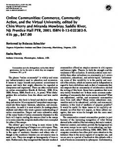
information of data i.e. the relationship between data points, whereas the original agreement measures that completely overlook the existence of these relationships, i.e edges. For more clarification see Figure 1.

(a) V

(b) U1

(c) U2

Fig. 1 Example for the benefits of the altered agreement indexes for graphs. Partitioning U1 and U 2 of the same graph with true partitioning V . Both partitionings have the exact same contingency table with V , {{5, 0}{1, 3}}, and therefore the same agreement value regardless of the agreement method used, however, U1 looks more similar to the true partitioning V , which is reflected in the adapted measure: in the degree weighted index, we have η(U1 , V ) = {{18, 0}{3, 9}} and η(U2 , V ) = {{14, 0}{7, 9}}. And in the edge based measure we have ξ(U1 , V ) = {{6, 0}{0, 3}} and ξ(U2 , V ) = {{4, 0}{0, 3}}.

4 Comparison Methodology and Results In this section, we first describe the our experimental settings. Then, we examine behaviour of different external indexes in comparing different community mining results. Next, we report the performances of the proposed community quality criteria in relative evaluation of communities.

4.1 Experiment Settings We have used three set of benchmarks as our datasets: Real, GN and LFR. The Real dataset consists of five well-known real-world benchmarks: Karate Club (weighted) by Zachary (Zachary 1977), Sawmill Strike data-set (Nooy et al. 2004), NCAA Football Bowl Subdivision (Girvan and Newman 2002), and Politician Books from Amazon (Krebs 2004). The GN and LFR datasets, each include 10 realizations of the GN and LFR synthetic benchmarks (Lancichinetti et al. 2008), which are the benchmarks widely in use for community mining evaluation. For each graph in our datasets, we generate different partitionings to sample the space of all possible partitionings. For doing so, given the perfect partitioning, we generate different randomized versions of the true partitioning by randomly merging and splitting communities and swapping nodes between them. The sampling procedure is described in more details in the supplementary materials. The set of the samples obtained covers the partitioning space in a way that it includes very poor to perfect samples.

20

Rabbany et al.

4.2 Agreement Indexes Experiments We have reviewed different agreement indexes used in external evaluation in Section 3.2. Here we first examine two characteristics of general clustering agreement indexes, then we illustrate our adopted indexes for graphs. 4.2.1 Bias of Unadjusted Indexes In Figure 2, we show the bias of the unadjusted indexes, where the average agreement of random partitionings to a true partitioning is plotted as a function of number of clusters5 . We can see that the average agreement increases for the unadjusted indexes when the number of clusters increases, while the adjusted rand index, ARI, is unaffected. Interestingly, we do not observe the same behaviour from AM I in all the datasets, while it is unaffected in football and GN datasets (where k  N ), it increases with the number of clusters in the strike and karate dataset (where k  N is not true).

(a) Karate

(b) Strike

(c) Football

(d) GN

Fig. 2 Necessity of adjustment of external indexes for agreement at chance. Here we generated 100 sample partitionings for each k, then for each sample, we computed its agreement with the true partitioning for that dataset. The average and variance of these agreements are plotted as a function of the number of clusters. We can see that the unadjusted measures of Rand, V I, Jaccard, F measure and N M I tend to increase/decrease as the the number of clusters in the random partitionings increases. While the Adjusted Rand Index (ARI) is unaffected and always returns zero for agreements at random. 5

Similar to the experiment performed in (Vinh et al. 2010).

Communities Validity

21

(a) Karate

(b) Strike

(c) Football

(d) GN

Fig. 3 Behaviour of different external indexes around the true number of clusters. We can see that the ARI exhibits a clear knee behaviour, i.e., its values are relatively lower for partitionings with too many or too few clusters. While others such as N M I and Rand comply less with this knee shape.

4.2.2 Knee Shape Figure 3, illustrates the behaviour of these criteria on different fragmentations of the ground-truth as a function of the number of clusters. The ideal behaviour is that the index should return relatively low scores for partitionings/fragmentations in which the number of clusters is much lower or higher than what we have in the ground-truth. In this figure, we can see that ARI exhibits this knee shape while N M I does not show this clearly. Table 1, reports the average correlation of these external indexes over these four datasets. Here we used the similar sampling procedure described before but we generate merge and split versions separately, so that the obtained samples are fragmentations of the ground-truth obtained from repeated merging or splitting. Refer to the supplementary materials for the detailed sampling procedure. There are different ways to compute the correlation between two vectors. The classic options are Pearson Product Moment coefficient or the Spearman’s Rank correlation coefficient. The reported results in our experiments are based on the Spearman’s Correlation, since we are interested on the correlation of rankings that an index provides for different partitionings and not the actual values of that index. However, the reported results mostly agree with the results obtained by using Pearson correlation, which are reported in

22

Rabbany et al.

Index ARI Rand NMI VI Jaccard AMI Fβ=2

ARI 1 0.73±0.18 0.67±0.07 -0.80±0.17 0.85±0.08 0.76±0.15 0.64±0.16

Rand 0.73±0.18 1 0.83±0.12 -0.46±0.42 0.41±0.32 0.71±0.11 0.13±0.46

NMI 0.67±0.07 0.83±0.12 1 -0.43±0.27 0.31±0.17 0.93±0.07 0.04±0.10

VI -0.80±0.17 -0.46±0.42 -0.43±0.27 1 -0.93±0.02 -0.54±0.27 -0.82±0.21

Jaccard 0.85±0.08 0.41±0.32 0.31±0.17 -0.93±0.02 1 0.46±0.28 0.90±0.13

AMI 0.76±0.15 0.71±0.11 0.93±0.07 -0.54±0.27 0.46±0.28 1 0.25±0.13

Fβ=2 0.64±0.16 0.13±0.46 0.04±0.10 -0.82±0.21 0.90±0.13 0.25±0.13 1

Table 1 Correlation between external indexes averaged for datasets of Figure 3, computed based on Spearman’s Correlation. Here we can see for example that ARI is behaves more similar to, has a higher correlation with, Adjusted Mutual Information,AM I, compared to Normalized Mutual Information, N M I. Index

ARI

ξ

1±0 0.571±0.142 0.956±0.031

0.571±0.142 1±0 0.623±0.133

ηw =d i i 0.956±0.031 0.623±0.133 1±0

ηw =t i i 0.819±0.135 0.572±0.169 0.876±0.097

ηw =c i i 0.838±0.087 0.45±0.109 0.777±0.106

NMI

ARI ξ ηw =d i i ηw =t i i ηw =c i i NMI

0.819±0.135 0.838±0.087 0.736±0.096

0.572±0.169 0.45±0.109 0.497±0.2

0.876±0.097 0.777±0.106 0.787±0.094

1±0 0.848±0.056 0.759±0.107

0.848±0.056 1±0 0.6±0.064

0.759±0.107 0.6±0.064 1±0

0.736±0.096 0.497±0.2 0.787±0.094

Table 2 Correlation between adopted external indexes on karate and strike datasets, computed based on Spearman’s Correlation. Here, ηwi =di , ηwi =ti , and ηwi =ci denote the weighted ARI where each node is weighted respectively by, its degree, the number of triangles it belongs to, or its clustering coefficient. The ξ, on the other hand, stands for the structural agreement based on number of edges (see Section 3.2.3 for more details).

the supplementary materialsavailable from: http://cs.ualberta.ca/∼rabbanyk/ criteriaComparison. 4.2.3 Graph Partitioning Agreement Indexes Finally, we examine the adopted versions of agreement measures described in Section 3.2.3. Figure 4 shows the constant baseline of these adopted criteria for agreements at random, and also the knee shape of the adopted measures around the true number of clusters, same as what we have for the original ARI. Therefore, one can safely apply one of these measures depending on the application at hand. Table 2 summarizes the correlation between each pair of the external measures. In the following we compare the performance of different quality indexes, defined in Section 3.1, in relative evaluation of clustering results.

4.3 Quality Indexes Experiments The performance of a criterion could be examined by how well it could rank different partitionings of a given dataset. More formally, consider we have a dataset d and a set of m different possible partitionings, i.e. P (d) = {pd1 , pd2 , . . . , pdm } Then, the performance of criterion c on dataset d could be determined by how much its values, Ic (d) = {c(pd1 ), c(pd2 ), . . . , c(pdm )}, correlate with the “goodness” of these partitionings. Assuming that the true partitioning (i.e. ground

Communities Validity

23

(a) Strike

(b) Football

(c) Strike

(d) Football

Fig. 4 Adopted agreement measures for graphs. On top we see that the adopted measures, specially the weighted indexes by degree (di ) and the number of triangles (ti ), are adjusted by chance, which can not be seen for the structural edge based version (ξ). The bottom figures illustrate the perseverance of the knee behaviour in the adopted measures.

truth) p∗d is known for dataset d, the “goodness” of partitioning pdi could be determined using partitioning agreement measure a. Hence, for dataset d with set of possible partitionings P (d), the external evaluation provides E(d) = {a(pd1 , p∗d ), a(pd2 , p∗d ), . . . , a(pdm , p∗d )}, where (pd1 , p∗d ) denotes the “goodness” of partitioning pd1 comparing to the ground truth. Then, the performance score of criterion c on dataset d could be examined by the correlation of its values Ic (d) and the values obtained from the external evaluation E(d) on different possible partitionings. Finally, the criteria are ranked based on their average performance score over a set of datasets. The following procedure summarizes our comparison approach. D ← {d1 , d2 , . . . , dn } for all dataset d ∈ D do P (d) ← {pd1 , pd2 , . . . , pdm } {generate m possible partitionings} E(d) ← {a(pd1 , p∗d ), a(pd2 , p∗d ), . . . , a(pdm , p∗d )} {compute the external scores} for all c ∈ Criteria do Ic (d) ← {c(pd1 ), c(pd2 ), . . . , c(pdm )} {compute the internal scores } scorec (d) ← correlation(E, I) {compute the correlation } end for end for Pn 1 scorec ← n scorec (d) {rank criteria based on their average scores} d=1

24

Rabbany et al.

Table 3 Statistics for sample partitionings of each real world dataset. For example, for the Karate Club dataset which has 2 communities in its ground truth, we have generated 100 different partitionings with average 3.82±1.51 clusters ranging from 2 to 7 and the “goodness” of the samples is on average 0.29±0.26 in terms of their ARI agreement. Dataset strike polboks karate football

K∗ 3 3 2 11

# 100 100 100 100

K 3.2±1.08∈[2,7] 4.36±1.73∈[2,9] 3.82±1.51∈[2,7] 12.04±4.8∈[4,25]

(a) ZIndex with Topological Overlap

ARI 0.45±0.27∈[0.01,1] 0.43±0.2∈[0.03,1] 0.29±0.26∈[-0.04,1] 0.55±0.22∈[0.16,1]

(b) Q modularity

(c) Point-Biserial with Pearson Correlation (d) Silhouette with Modularity Proximity Fig. 5 Visualization of correlation between an external agreement measure and some relative quality criteria for Karate dataset. The x axis indicates different random partitionings, and the y axis indicates the value of the index. While, the blue/darker line represents the value of the external index for the given partitioning and the red/lighter line represents the value that the criterion gives for the partitioning. Please note that the value of criteria are not generally normalized and in the same range as the external indexes, in this figure ARI. For the sake of illustration therefore, each criterion’s values are scaled to be in the same range as of the external index.

4.3.1 Results on Real World Datasets Table 3 shows general statistics of our real world datasets and their generated samples. We can see that the randomized samples cover the space of partitionings according to their external index range. Figure 5 exemplifies how different criteria exhibit different correlations with the external index. It visualizes the correlation between few selected relative indexes and an external index for one of our datasets listed in Table 3. Similar

Communities Validity

25

analysis is done for all 4 datasets × 645 criteria (combination of relative indexes and distances variations) × 5 external indexes, which produced over 12900 such correlations. The top ranked criteria based on their average performance over these datasets are summarized in Table 4. Based on these results, ZIndex when used with almost all of the proximity measures, such as Topological Overlap (TO), Pearson Correlation Similarity (PC ) or Intersection Closeness (IC ); has a higher correlation with the external index comparing to the modularity Q. And this is true regardless of the choice of ARI as the external index, since it is ranked above Q also by other external indexes, e.g. NMI and NMI. Other criteria, on the other hand, are all ranked after the modularity Q, except the CIndex SP. One may conclude based on this experiment that ZIndex is a more accurate evaluation criterion comparing to Q. We can also examine the ranking of different proximity measures in this table. For example, we can see that the Number of Paths of length 2, N P 2, performs better than length 3, N P 3; and that the exponential combination of N P E performs better than linear, N P L, and uniform, N P , alternatives. The correlation between a criterion and an external index depends on how close the randomized partitionings are from the true partitioning of the ground truth. This can be seen in Figure 5. For example, SWC1 (Silhouette with Criterion where distance of a node to a community is computed by its distance to the centroid of that community) with the Modularity M proximity agrees strongly with the external index in samples with higher external index value, i.e. closer to the ground truth, but not on further samples. We can also see the similar pattern in the Point-Biserial with PC proximity. With this in mind, we have divided the generated clustering samples into three sets of easy, medium and hard samples and re-ranked the criteria in each of these settings. Since the external index determines how far a sample is from the optimal result, the samples are divided into three equal length intervals according to the range of the external index. Table 5, reports the rankings of the top criteria in each of these three settings. We can see that these average results support our earlier hypothesis, i.e., when considering partitionings near or medium far from the true partitioning, PB’ PC is between top criteria, while its performance drops significantly for samples very far from the ground truth. 4.3.2 Synthetic Benchmarks Datasets Similar to the last experiment, Table 7 reports the ranking of the top criteria according to their average performance on synthesized datasets of Table 6. Based on which, ZIndex overall outperforms other criteria including the modularity Q, this is more significant in ranking finner partitionings, near optimal; while it is less significant in ranking poor partitionings. The LFR generator can generate networks with different levels of difficulty for the partitioning task, by changing how well separated the communities are in the ground truth. To examine the effect of this difficulty parameter, we have ranked the criteria for different values of this parameter. We observed that modularity Q becomes the overall superior criterion for synthetic benchmarks

26

Rabbany et al.

Table 4 Overall ranking of criteria on the real world datasets, based on the average Spearman’s correlation of criteria with the ARI external index, ARIcorr . Ranking based on correlation with other external indexes is also reported. The full ranking of the 654 criteria, which is not reported here due to space limit, can be accessed in the supplementary materials. Rank 1 2 3 4 5 6 7 8 9 10 11 12 13 14 15 16 17 18 19 20 21 22 23 24 25 26 27 28 29 30 31 32 33 34 35 36 37 38 39 40 41 42 43 44 45 46 47 48 49 50

Criterion ZIndex’ TO ZIndex’ PˆC ˆC ZIndex’ N P ZIndex’ IC2 ZIndex’ TˆO ˆO ZIndex’ N P ZIndex’ ICV2 ZIndex’ PC ZIndex’ IC3 ˆ ZIndex’ N OV ZIndex’ IC1 ZIndex’ NPE2.0 ZIndex’ NOV ZIndex’ ICV1 ZIndex’ N P ˆE2.0 ZIndex’ NPL2.0 ZIndex’ M ZIndex’ ICV3 ZIndex’ NP2.0 ZIndex’ N P ˆL2.0 ZIndex’ N Pˆ2.0 ZIndex’ NˆO ZIndex’ NO ZIndex’ MˆM CIndex SP ZIndex’ N P ˆL3.0 ZIndex’ N Pˆ3.0 ZIndex’ N P ˆE3.0 ˆ ZIndex AR ZIndex’ NPE3.0 ZIndex’ NPL3.0 ZIndex SP ZIndex’ NP3.0 ZIndex AR ZIndex’ A ZIndex’ MD ˆ ZIndex’ A Q CIndex’ NPE3.0 CIndex’ ICV3 CIndex AR ˆ CIndex AR CIndex’ N P ˆE3.0 ZIndex’ MˆD SWC0 IC1 SWC0 IC2 SWC0 NO SWC0 IC3 SWC0 NOV SWC0 ICV1

ARIcorr 0.925±0.018 0.923±0.012 0.923±0.012 0.922±0.024 0.922±0.016 0.921±0.014 0.919±0.04 0.918±0.018 0.918±0.039 0.915±0.014 0.912±0.02 0.911±0.03 0.91±0.023 0.91±0.023 0.91±0.025 0.909±0.02 0.908±0.028 0.908±0.057 0.907±0.021 0.906±0.022 0.906±0.022 0.905±0.022 0.904±0.034 0.903±0.037 0.9±0.02 0.899±0.032 0.899±0.033 0.899±0.048 0.898±0.035 0.897±0.052 0.897±0.038 0.895±0.036 0.895±0.039 0.895±0.039 0.894±0.045 0.894±0.048 0.891±0.05 0.878±0.034 0.876±0.054 0.869±0.069 0.864±0.031 0.861±0.032 0.858±0.07 0.856±0.101 0.847±0.09 0.838±0.092 0.837±0.106 0.819±0.104 0.814±0.094 0.814±0.094

Rand 9 2 3 8 10 6 18 4 19 11 5 26 12 13 23 24 25 29 20 21 22 16 7 17 1 30 33 31 14 35 36 28 37 15 32 34 27 45 43 44 40 42 47 38 41 49 39 57 52 53

Jaccard 148 197 198 182 153 204 163 207 165 213 235 168 225 226 184 202 149 176 212 216 217 253 250 233 251 200 196 205 264 187 170 215 166 255 158 179 241 110 9 4 268 266 8 323 108 11 146 7 26 27

NMI 9 2 1 5 8 3 12 10 15 6 13 21 18 19 22 14 26 28 16 17 20 11 23 24 31 27 29 35 30 39 32 40 34 36 38 33 37 45 4 7 42 41 25 43 46 50 48 58 54 55

AMI 7 2 1 3 8 4 10 11 12 9 20 15 21 22 19 13 23 25 14 17 18 16 31 30 42 24 27 33 36 34 28 41 29 38 35 32 37 44 6 5 40 39 26 45 47 49 50 52 56 57

Communities Validity

27

Table 5 Difficulty analysis of the results: considering ranking for partitionings near optimal ground truth, medium far and very far. Reported result are based on ARI and the Spearman’s correlation. Rank 1 2 3 4 5 6 7 8 9 10 11 12

36 37 38 39 40 Rank 1 2 3 4 5 6 7 8 9 10 11 12

29 30

31 46 Rank 1 2 3 4 5 6 7 8 9 10 11 12

30 31 32 33 34

117

Near Optimal Samples ARIcorr Rand 0.851±0.081 1 0.851±0.081 2 0.847±0.084 18 0.845±0.088 3 0.845±0.065 30 0.842±0.082 10 0.839±0.084 4 0.835±0.093 11 0.835±0.09 9 0.834±0.089 13 0.834±0.089 7 0.834±0.095 5 .. . ZIndex’ M 0.763±0.139 33 Q 0.762±0.166 39 DB ICV3 0.757±0.126 37 DB IC3 0.753±0.176 35 PB’ PC 0.753±0.289 45 Medium Far Samples Criterion ARIcorr Rand ZIndex’ TO 0.775±0.087 5 ZIndex’ TˆO 0.771±0.091 6 ZIndex’ IC3 0.768±0.134 2 ZIndex’ ICV2 0.766±0.124 3 ZIndex’ NPL3.0 0.762±0.079 12 ZIndex’ ICV3 0.757±0.12 4 ZIndex’ NP3.0 0.756±0.085 15 ZIndex’ PˆC 0.755±0.122 9 ˆC ZIndex’ N P 0.755±0.122 11 ZIndex’ NPE2.0 0.753±0.107 10 ZIndex’ NPE3.0 0.746±0.093 8 ˆO ZIndex’ N P 0.744±0.123 14 .. . ZIndex’ MˆM 0.694±0.168 31 Q 0.69±0.151 58 .. . ZIndex’ A 0.69±0.144 34 PB’ PC 0.623±0.06 112 Far Far Samples Criterion ARIcorr Rand ZIndex’ ICV2 0.724±0.066 36 ZIndex’ IC3 0.72±0.062 40 ZIndex’ ICV3 0.717±0.059 47 ZIndex’ IC2 0.715±0.072 35 ZIndex’ TO 0.706±0.064 49 ˆO ZIndex’ N P 0.704±0.076 44 ZIndex’ TˆO 0.704±0.062 51 ZIndex’ NPE2.0 0.701±0.057 55 ˆC ZIndex’ N P 0.698±0.083 45 ZIndex’ PˆC 0.697±0.083 46 ZIndex’ N P ˆE2.0 0.688±0.047 57 ZIndex’ NPL2.0 0.688±0.072 58 .. . ZIndex’ IC1 0.655±0.132 43 ZIndex’ NˆO 0.651±0.106 52 Q 0.643±0.033 86 ZIndex’ NO 0.638±0.158 38 ZIndex’ MD 0.63±0.099 78 .. . PB’ PC 0.372±0.126 197 Criterion ˆC ZIndex’ N P ZIndex’ PˆC ZIndex SP ˆO ZIndex’ N P DB ICV2 ZIndex’ N P ˆE3.0 ZIndex’ ICV3 ˆ ZIndex’ N OV ZIndex’ TˆO ZIndex’ N P ˆE2.0 ZIndex’ TO ZIndex’ IC2

Jaccard 3 4 2 9 1 5 20 14 10 8 16 23

NMI 4 3 8 6 31 2 20 15 7 1 11 18

AMI 5 3 8 6 30 2 21 15 7 1 11 18

29 21 35 36 26

30 41 38 39 71

31 41 36 39 71

Jaccard 361 386 372 370 349 376 354 417 418 373 369 437

NMI 22 19 16 2 28 21 29 4 3 14 24 5

AMI 20 17 13 2 27 19 28 4 3 14 24 5

458 70

40 79

32 72

366 28

58 200

54 157

Jaccard 520 523 511 540 519 547 522 505 552 553 521 529

NMI 4 11 23 3 16 1 13 15 6 9 24 12

AMI 9 19 25 6 14 3 5 7 10 11 23 4

566 567 444 572 513

34 22 50 38 43

40 26 45 47 41

170

159

129

28

Rabbany et al.

Table 6 Statistics for sample partitionings of each synthetic dataset. The benchmark generation parameters: 100 nodes with average degree 5 and maximum degree 50, where size of each community is between 5 and 50 and mixing parameter is 0.1. Dataset network1 network2 network3 network4 network5 network6 network7 network8 network9 network10

K∗ 4 3 2 7 2 5 4 5 5 6

# 100 100 100 100 100 100 100 100 100 100

K 5.26±2.45∈[2,12] 4±1.7∈[2,8] 4±1.33∈[2,6] 10.68±3.3∈[4,19] 4.68±1.91∈[2,9] 5.98±2.63∈[2,14] 6.62±2.72∈[2,12] 5.8±2.45∈[2,12] 6.54±2.08∈[3,11] 8.88±2.74∈[4,15]

ARI 0.45±0.18∈[0.13,1] 0.47±0.23∈[0.06,1] 0.36±0.22∈[0.07,1] 0.69±0.21∈[0.25,1] 0.32±0.22∈[-0.01,1] 0.52±0.21∈[0.12,1] 0.52±0.22∈[0.11,1] 0.55±0.22∈[0.15,1] 0.64±0.2∈[0.25,1] 0.59±0.19∈[0.21,1]

with higher level of mixed communities (.3 ≤ µ ≤ .5). Table 8 reports the overall ranking of the criteria for a difficult set of datasets that have high mixing parameter. We can see that although Q is the overall superior criterion, ZIndex still significantly outperforms Q in ranking finer partitionings. Results for other settings are available in the supplementary materials. In short, the relative performances of different criteria depends on the difficulty of the network itself, as well as how far we are sampling from the ground truth. Altogether, choosing the right criterion for evaluating different community mining results depends both on the application, i.e., how well-separated communities might be in the given network, and also on the algorithm that produces these results, i.e., how fine the results might be. For example, if the algorithms is producing high quality results close to the optimal, modularity Q might not distinguish the good and bad partitionings very well. While if we are choosing between mixed and not well separated clusterings, it is the superior criterion 6 .

5 Conclusion In this article, we examined different approaches for evaluating community mining results. Particularly we examined different external and relative measures defined for clustering validity and adopted these for the inter-related data. The main contribution is our generalization for well-known clustering validity criteria originally used as quantitative measures for evaluating quality of clusters of data points represented by attributes. The first reason of this generalization is to adapt these criteria in the context of community mining of interrelated data. The only commonly used criterion to evaluate the goodness of detected communities in a network is the modularity Q. Providing more validity criteria can help researchers to better evaluate and compare community mining results in different settings. Also, these adapted validity criteria 6 Please note that these results and criteria are different from our earlier work (Rabbany et al. 2012), particularly, ZIndex is defined differently in this paper.

Communities Validity

29

Table 7 Overall ranking and difficulty analysis of the synthetic results. Here communities are well-separated with mixing parameter of .1. Similar to the last experiment, reported result are based on AMI and the Spearman’s correlation. Rank 1 2 3 4 5 6 7 8 9 10 11 12 13 14 15

Criterion ZIndex’ ICV2 ZIndex’ IC3 ZIndex’ IC2 ZIndex’ PˆC ˆC ZIndex’ N P ZIndex’ ICV3 ˆO ZIndex’ N P ZIndex’ TˆO ˆ ZIndex’ N OV ZIndex’ TO ZIndex’ PC ZIndex’ N P ˆE2.0 ZIndex’ NPE2.0 ZIndex’ NOV ZIndex’ ICV1

29 30 31

ZIndex’ NPL3.0 Q ZIndex’ NP3.0

Rank 1 2 3 4 5 6 7 8 9

Criterion ZIndex’ IC2 CIndex’ ICV2 ZIndex’ IC3 CIndex’ ICV3 ZIndex’ ICV2 ˆ ZIndex’ A CIndex’ IC3 ZIndex’ A ZIndex’ MˆM

206 207

SWC1’ NˆO Q

Rank 1 2 3 4 5 6 7 8 9 10

Criterion ZIndex’ ICV2 ZIndex’ IC2 ZIndex’ IC3 ZIndex’ ICV3 ZIndex’ PˆC ˆC ZIndex’ N P CIndex’ ICV3 ˆO ZIndex’ N P ZIndex’ TˆO ZIndex’ TO

37

Q

Rank 1 2 3 4 5

Criterion ZIndex’ ICV2 ZIndex’ IC3 ZIndex’ TO ZIndex’ ICV3 ZIndex’ TˆO

30 31 32

ZIndex’ M Q ZIndex SP

Overall Results ARIcorr Rand 0.96±0.029 5 0.958±0.028 4 0.958±0.033 1 0.953±0.04 3 0.953±0.04 2 0.953±0.027 8 0.951±0.041 6 0.949±0.045 13 0.949±0.042 7 0.948±0.046 16 0.947±0.043 10 0.947±0.042 11 0.946±0.043 17 0.941±0.047 14 0.941±0.047 15 .. . 0.895±0.072 31 0.893±0.046 33 0.89±0.076 32 Near Optimal Results ARIcorr Rand 0.826±0.227 2 0.822±0.132 7 0.821±0.232 1 0.818±0.237 4 0.816±0.232 3 0.813±0.225 5 0.8±0.2 31 0.795±0.177 30 0.794±0.221 9 .. . 0.591±0.179 225 0.589±0.161 222 Medium Far Results ARIcorr Rand 0.741±0.177 4 0.738±0.181 1 0.728±0.188 5 0.721±0.177 8 0.719±0.204 3 0.719±0.204 2 0.713±0.151 28 0.709±0.205 7 0.703±0.216 12 0.702±0.217 14 .. . 0.62±0.139 42 Far Far Results ARIcorr Rand 0.834±0.062 9 0.832±0.06 7 0.825±0.098 22 0.823±0.063 12 0.823±0.096 18 .. . 0.638±0.151 31 0.581±0.155 95 0.58±0.158 72

Jaccard 32 42 58 78 79 44 83 60 90 50 77 68 51 95 96

NMI 3 2 1 6 7 4 9 17 8 21 16 13 20 18 19

AMI 3 2 1 6 7 5 9 17 8 21 15 13 20 18 19

121 33 130

38 26 39

37 22 39

Jaccard 10 1 16 9 18 19 2 20 33

NMI 4 11 5 3 7 2 13 6 1

AMI 6 7 9 5 10 2 8 4 1

194 198

244 138

233 110

Jaccard 231 247 252 258 285 286 21 278 240 239

NMI 22 16 18 21 30 31 33 32 42 45

AMI 22 20 21 23 35 36 27 38 48 53

167

56

47

Jaccard 464 469 423 458 446

NMI 5 4 29 6 27

AMI 3 2 27 6 25

537 368 539

9 69 25

4 32 29

30

Rabbany et al.

Table 8 Overall ranking of criteria based on AMI & Spearman’s Correlation on the synthetic benchmarks with the same parameters as in Table 6 but much higher mixing parameter, .4. We can see that in these settings, modularity Q overall outperforms the ZIndex while the latter is significantly better in differentiating finer results near optimal. Rank 1 2 3 4 5 6 7 8 9 10

Criterion Q ZIndex’ M ZIndex’ A ZIndex’ MˆM ˆ ZIndex’ A ZIndex’ PˆC ˆC ZIndex’ N P ˆO ZIndex’ N P ZIndex’ TˆO ˆ ZIndex’ N OV

Rank 1 2 3 4 5 6 7 8 9 10

Criterion ZIndex’ M ZIndex’ A ZIndex’ MˆM ˆ ZIndex’ A Q ASWC0 N P ˆL2.0 SWC0 N P ˆL2.0 ZIndex’ N P ˆE2.0 ASWC0 SP ZIndex’ N P ˆL2.0

Rank 1 2 3 4 5 6 7 8 9 10 Rank 1 2 3 4 5 6 7 8 9 10

Overall Results ARIcorr Rand 0.854±0.039 11 0.839±0.067 2 0.813±0.071 4 0.785±0.115 1 0.767±0.101 3 0.748±0.19 5 0.748±0.19 6 0.745±0.191 7 0.738±0.197 13 0.738±0.197 8

Near Optimal Results ARIcorr Rand 0.825±0.105 1 0.8±0.184 2 0.768±0.166 3 0.76±0.192 4 0.72±0.209 34 0.719±0.248 22 0.718±0.247 23 0.714±0.259 5 0.71±0.286 28 0.702±0.261 6 Medium Far Results Criterion ARIcorr Rand Q 0.578±0.124 106 ˆC CIndex’ N P 0.522±0.146 154 CIndex’ PˆC 0.521±0.146 155 ˆO CIndex’ N P 0.519±0.142 176 ˆ CIndex’ N OV 0.501±0.14 209 ZIndex’ M 0.498±0.199 4 CIndex’ IC2 0.492±0.146 227 CIndex’ ICV2 0.483±0.193 149 CIndex’ IC3 0.478±0.191 187 CIndex’ TO 0.478±0.175 179 Far Far Results Criterion ARIcorr Rand ZIndex’ PˆC 0.527±0.169 61 ˆC ZIndex’ N P 0.527±0.169 62 Q 0.523±0.192 128 ZIndex’ M 0.522±0.121 77 ˆO ZIndex’ N P 0.518±0.168 63 ˆ ZIndex’ N OV 0.515±0.166 60 ZIndex’ TˆO 0.489±0.171 78 ZIndex’ N P ˆE2.0 0.481±0.168 79 ZIndex’ MˆM 0.48±0.15 30 ZIndex’ NˆO 0.48±0.17 43

Jaccard 1 5 11 63 86 108 109 110 88 134

NMI 4 1 3 2 5 7 8 9 16 10

AMI 2 1 3 4 5 7 8 9 15 10

Jaccard 1 2 4 6 3 8 9 21 5 29

NMI 1 2 3 4 34 5 6 7 29 13

AMI 1 2 3 4 34 5 6 8 26 18

Jaccard 22 12 13 5 4 364 9 79 43 31

NMI 3 78 79 120 142 2 176 119 148 204

AMI 1 69 70 100 135 2 173 115 146 203

Jaccard 501 502 73 465 504 518 485 491 553 552

NMI 5 6 93 8 10 11 15 24 2 7

AMI 4 5 25 2 6 7 9 14 3 8

Communities Validity

31

can be further used as objectives to design new community mining algorithms. Our generalized formulation is independent of any particular distance measure unlike most of the original clustering validity criteria that are defined based on the Euclidean distance. The adopted versions therefore could be used as community criteria when plugged in with different graph distances. In our experiments, several of these adopted criteria exhibit high performances on ranking different partitionings of a given dataset, which makes them possible alternatives for the Q modularity. However, a more careful examination is needed as the rankings depends significantly on the experimental settings and the criteria should be chosen based on the application.

Acknowledgment The authors are grateful for the support from Alberta Innovates Centre for Machine Learning and NSERC. Ricardo Campello also acknowledges the financial support of Fapesp and CNPq.

References Albatineh, A. N., Niewiadomska-Bugaj, M., and Mihalko, D. (2006). On similarity indices and correction for chance agreement. Journal of Classification, 23:301–313. 10.1007/s00357-006-0017-z. Calinski, T. and Harabasz, J. (1974). A dendrite method for cluster analysis. Communications in Statistics-theory and Methods, 3:1–27. Chen, J., Za¨ıane, O. R., and Goebel, R. (2009a). Detecting communities in large networks by iterative local expansion. In International Conference on Computational Aspects of Social Networks, pages 105–112. Chen, J., Za¨ıane, O. R., and Goebel, R. (2009b). Detecting communities in social networks using max-min modularity. In SIAM International Conference on Data Mining, pages 978–989. Clauset, A. (2005). Finding local community structure in networks. Physical Review E (Statistical, Nonlinear, and Soft Matter Physics), 72(2):026132. Dalrymple-Alford, E. C. (1970). Measurement of clustering in free recall. Psychological Bulletin, 74:32–34. Danon, L., Guilera, A. D., Duch, J., and Arenas, A. (2005). Comparing community structure identification. Journal of Statistical Mechanics: Theory and Experiment, (09):09008. Davies, D. L. and Bouldin, D. W. (1979). A cluster separation measure. Pattern Analysis and Machine Intelligence, IEEE Transactions on, PAMI1(2):224 –227. Dunn, J. C. (1974). Well-separated clusters and optimal fuzzy partitions. Journal of Cybernetics, 4(1):95–104. Fortunato, S. (2010). Community detection in graphs. Physics Reports, 486(35):75–174.

32

Rabbany et al.

Fortunato, S. and Barth´elemy, M. (2007). Resolution limit in community detection. Proceedings of the National Academy of Sciences, 104(1):36–41. Girvan, M. and Newman, M. E. J. (2002). Community structure in social and biological networks. Proceedings of the National Academy of Sciences, 99(12):7821–7826. Gustafsson, M., H¨ ornquist, M., and Lombardi, A. (2006). Comparison and validation of community structures in complex networks. Physica A Statistical Mechanics and its Applications, 367:559–576. Halkidi, M., Batistakis, Y., and Vazirgiannis, M. (2001). On clustering validation techniques. Journal of Intelligent Information Systems, 17:107–145. Hubert, L. and Arabie, P. (1985). Comparing partitions. Journal of Classification, 2:193–218. Hubert, L. J. and Levin, J. R. (1976). A general statistical framework for assessing categorical clustering in free recall. Psychological Bulletin, 83:1072– 1080. Kenley, E. C. and Cho, Y.-R. (2011). Entropy-based graph clustering: Application to biological and social networks. In IEEE International Conference on Data Mining. Krebs, V. (2004). Books about us politics. http://www.orgnet.com/. Lancichinetti, A. and Fortunato, S. (2009). Community detection algorithms: A comparative analysis. Physical Review E, 80(5):056117. Lancichinetti, A., Fortunato, S., and Radicchi, F. (2008). Benchmark graphs for testing community detection algorithms. Physical Review E, 78(4):046110. Leskovec, J., Lang, K. J., and Mahoney, M. (2010). Empirical comparison of algorithms for network community detection. In International conference on World wide web, pages 631–640. Luo, F., Wang, J. Z., and Promislow, E. (2008). Exploring local community structures in large networks. Web Intelligence and Agent Systems, 6:387– 400. Manning, C. D., Raghavan, P., and Schtze, H. (2008). Introduction to Information Retrieval. Cambridge University Press, New York, NY, USA. Meil, M. (2007). Comparing clusteringsan information based distance. Journal of Multivariate Analysis, 98(5):873 – 895. Milligan, G. and Cooper, M. (1985). An examination of procedures for determining the number of clusters in a data set. Psychometrika, 50(2):159–179. Newman, M. E. J. (2006). Modularity and community structure in networks. Proceedings of the National Academy of Sciences, 103(23):8577–8582. Newman, M. E. J. and Girvan, M. (2004). Finding and evaluating community structure in networks. Physical Review E, 69(2):026113. Nooy, W. d., Mrvar, A., and Batagelj, V. (2004). Exploratory Social Network Analysis with Pajek. Cambridge University Press. Orman, G. K. and Labatut, V. (2010). The effect of network realism on community detection algorithms. In Proceedings of the 2010 International Conference on Advances in Social Networks Analysis and Mining, ASONAM ’10, pages 301–305.

Communities Validity

33

Orman, G. K., Labatut, V., and Cherifi, H. (2011). Qualitative comparison of community detection algorithms. In International Conference on Digital Information and Communication Technology and Its Applications, volume 167, pages 265–279. Pakhira, M. and Dutta, A. (2011). Computing approximate value of the pbm index for counting number of clusters using genetic algorithm. In International Conference on Recent Trends in Information Systems, pages 241 –245. Palla, G., Derenyi, I., Farkas, I., and Vicsek, T. (2005). Uncovering the overlapping community structure of complex networks in nature and society. Nature, 435(7043):814–818. Porter, M. A., Onnela, J.-P., and Mucha, P. J. (2009). Communities in Networks. ArXiv e-prints. Rabbany, R., Chen, J., and Za¨ıane, O. R. (2010). Top leaders community detection approach in information networks. In SNA-KDD Workshop on Social Network Mining and Analysis. Rabbany, R., Takaffoli, M., Fagnan, J., Zaiane, O., and Campello, R. (2012). Relative validity criteria for community mining algorithms. In Advances in Social Networks Analysis and Mining (ASONAM), 2012 International Conference on. Rabbany, R. and Za¨ıane, O. R. (2011). A diffusion of innovation-based closeness measure for network associations. In IEEE International Conference on Data Mining Workshops, pages 381 –388. Ravasz, E., Somera, A. L., Mongru, D. A., Oltvai, Z. N., and Barabsi, A.L. (2002). Hierarchical organization of modularity in metabolic networks. Science, 297(5586):1551–1555. Rosvall, M. and Bergstrom, C. T. (2007). An information-theoretic framework for resolving community structure in complex networks. Proceedings of the National Academy of Sciences, 104(18):7327–7331. Rosvall, M. and Bergstrom, C. T. (2008). Maps of random walks on complex networks reveal community structure. Proceedings of the National Academy of Sciences, 105(4):1118–1123. Rousseeuw, P. (1987). Silhouettes: a graphical aid to the interpretation and validation of cluster analysis. Journal of Computational and Applied Mathematics, 20(1):53–65. Theodoridis, S. and Koutroumbas, K. (2009). Cluster validity. In Pattern Recognition, chapter 16. Elsevier Science, 4 edition. Vendramin, L., Campello, R. J. G. B., and Hruschka, E. R. (2010). Relative clustering validity criteria: A comparative overview. Statistical Analysis and Data Mining, 3(4):209–235. Vinh, N. X., Epps, J., and Bailey, J. (2009). Information theoretic measures for clusterings comparison: is a correction for chance necessary? In Proceedings of the 26th Annual International Conference on Machine Learning, ICML ’09, pages 1073–1080, New York, NY, USA. ACM. Vinh, N. X., Epps, J., and Bailey, J. (2010). Information theoretic measures for clusterings comparison: Variants, properties, normalization and correction

34

Rabbany et al.

for chance. Journal of Machine Learning Research, 11:2837–2854. Wasserman, S. and Faust, K. (1994). Social Network Analysis: Methods and Applications. Cambridge University Press. Wu, J., Xiong, H., and Chen, J. (2009). Adapting the right measures for kmeans clustering. In Proceedings of the 15th ACM SIGKDD international conference on Knowledge discovery and data mining, KDD ’09, pages 877– 886, New York, NY, USA. ACM. Zachary, W. W. (1977). An information flow model for conflict and fission in small groups. Journal of Anthropological Research, 33:452–473.