Compact Forbidden-set Routing Bruno Courcelle∗
Andrew Twigg†
Abstract We study labelling schemes for X-constrained path problems. Given a graph (V, E) and X ⊆ V , a path is X-constrained if all intermediate vertices avoid X. We study the problem of assigning labels J(x) to vertices so that given {J(x) : x ∈ X} for any X ⊆ V , we can route on the shortest X-constrained path between x, y ∈ X. This problem is motivated by Internet routing, where the presence of routing policies means that shortest-path routing is not appropriate. For graphs of tree width k, we give a routing scheme using routing tables of size O(k2 log2 n). We introduce m-clique width, generalizing clique width, to show that graphs of m-clique width k also have a routing scheme using size O(k2 log2 n) tables.
Keywords: Algorithms, labelling schemes, compact routing.
1
Introduction
Given a graph G = (V, E) where each vertex u ∈ V has a forbidden set S(u) ⊆ V , a compact forbidden-set routing scheme is a compact routing scheme where all routes from u are shortest paths in the (possibly disconnected) graph G \ S(u). The problem is motivated by Internet routing, where nodes (routers) can independently set routing policies that assign costs to paths, thus making the shortest path not necessarily the most desirable. Shortest-path routing is well-understood, for example Thorup and Zwick [17] have given a compact ˜ √n) size tables, which is almost optimal for stretchrouting scheme using O( 3 paths. On the other hand, very little is known about the complexity of forbidden-set routing. The only known algorithms for policy routing (such as BGP) use Bellman-Ford iteration to construct so-called stable routing trees – for each destination, a tree is rooted at that destination and packets are forwarded along it. Varadhan et al.[18] showed that the policies may conflict, forcing the algorithm to not converge. For general policies, Griffin et al.[11] showed that deciding if it will converge is NP-complete, and Feigenbaum and Karger et al.[9] showed that NP-completeness still holds for forbidden-set policies. This motivates the problem of designing efficient routing schemes that do not suffer from non-convergence, for simple classes of policy such as forbidden-set. ∗ LaBRI,
Bordeaux 1 University and CNRS, email:
[email protected] Laboratory, Cambridge University, email:
[email protected]
† Computer
1
2
Preliminaries
Let G = (V, E) be an undirected graph and X ⊆ V a set of vertices (the extension to directed graphs is straightforward), and F be a set of edges. An (X, F )-constrained path is a path in G that does not use the edges of F and with no intermediate vertex in X (or simply X-constrained if F is empty). We denote by G[Z] the subgraph of G induced by a set of vertices Z. We denote by G+ [Z] the graph consisting of G[Z] and weighted edges where an edge between x and y has weight d iff d is the length of a shortest path in G between x and y of length at least 2 with no intermediate vertex in Z. Between two vertices, one may have one edge without value and another one with value at least 2. If we know the graph G+ [Z], if X ⊆ Z and every edge of F has its two ends in Z, we can get the length of a shortest (X, F )-constrained path in G between any x, y ∈ Z. The graph G+ [Z] captures the separator structure of G since there is no edge between x, y in G+ [X ∪ {x, y}] iff X is a separator of x, y in G, thus the problem can be seen as constructing a distributed encoding of the separators of a graph. In all cases we say that we consider a constrained path problem. Our objective is to label each vertex x of G by a label J(x), as short as possible, in such a way that G+ [Z] can be constructed from {J(x) : x ∈ Z}. If we can determine the lengths of shortest (X, F )-constrained paths from {J(x) : x ∈ Z}, where X ⊆ Z and every edge of F has its two ends in Z, then we call J(x) an (X, F )-constrained distance labelling. The graph problem ‘is there an X-constrained path from x to y?’ is monadic second-order definable, so the result of Courcelle and Vanicat [8] implies that graphs of bounded clique width have a labelling with labels of O(log n) bits. However, the constant factor is a tower of exponentials in cwd(G) and is impractical. Our main result is a labelling scheme with labels of size O(k 2 log2 (n)) where k is a bound on the m-clique width (mcwd) of the graph, a generalization of clique width that we will introduce. Since graphs with tree width (twd) k have mcwd at most k + 3, and graphs with clique width (cwd) k have mcwd at most k, the results follow for the case of tree width and clique width. Table 1 in [12] shows that the networks of some important major internet providers are of small tree width, between 10 and 20 and hence our constraint of dealing with graphs of small tree width or clique width is somehow realistic. The labeling works as follows: given vertices between which we want to determine shortest paths and a set Z ⊆ V , we construct from {J(x) : x ∈ Z} the weighted graph G+ [Z]. Then we can answer queries about 4-tuples (x, y, X, F ) such that X ∪ {x, y} ⊆ Z and every edge of F has its two ends in Z by using only G+ [Z] : in particular the length of a shortest (X, F )-constrained path. The idea is not to repeat for each query the construction of G+ [Y ] for some set Y . Our notation follows Courcelle and Vanicat [8]. For a finite set C of constants, a finite set F of binary function symbols, we let T (F, C) be the set of finite well-formed terms over these two sets (terms will be discussed as labelled trees). The size |t| of a term t is the number of occurrences of symbols 2
from C ∪ F . Its height ht(t) is 1 for a constant and 1 + max{ht(t1 ), ht(t2 )} for t = f (t1 , t2 ). Let a be a real number. A term t is said to be a-balanced if ht(t) ≤ a log |t| (all logarithms are to base 2). Let t in T (Fk , Ck ) and G = val(t), the graph obtained by evaluating t. For a node u in t, val(t/u) is the subgraph represented by evaluating the subterm rooted at u.
3
The case of tree width
Before presenting our main result on m-clique width graphs, we describe a labelling scheme for graphs of tree width k. A graph having tree width k can be expressed as the nondisjoint union of graphs of size k + 1, arranged as nodes in a tree such that the set of tree nodes containing some graph vertex forms a connected subtree of the tree (often called a tree decomposition). We shall work with a different, algebraic representation of graphs.
3.1
Balanced tree width expressions
Every graph of tree width k can be represented by an algebraic expression (term). A j-source graph is a graph with at most j distinguished vertices called sources, each tagged with a unique label from {1, . . . , j}. Courcelle [5, 1] shows that a graph has tree width k iff it is isomorphic to val(t) for some term t whose leaves are (k + 1)-source graphs and where every non-leaf node is labelled with one of the following operations, as illustrated in Figure 1. • Parallel composition: The (k + 1)-source graph (G // H) is obtained from the disjoint union of (k + 1)-source graphs G and H where sources having the same label are fused together into a single vertex. • Erasure: For a ∈ {1, . . . , k + 1}, the unary operation fga (G) erases the label a and the corresponding source in G is no longer a source vertex. As in Courcelle and Vanicat[8], we combine a parallel composition and a sequence of erasure operations to obtain a single binary operation, e.g. // fga,b . The term tree can be constructed given a tree decomposition of the graph – Corollary 2.1.1 of Courcelle [5] shows that given a tree decomposition of width k of a graph, it is possible to construct in linear time a term tree using at most k + 1 source labels. The nodes of the term tree are the bags of the tree decomposition; hence the height and degree are unchanged. The following result of Bodlaender shows how to obtain a balanced tree width expression with a small increase in tree width. Lemma 1 (Bodlaender [2]) Given a tree decomposition of width k and a graph G with n vertices, one can compute a binary tree decomposition of G of height at most 2 log5/4 (2n) and width at most 3k + 2 in time O(n).
3
Parallel composition: 1
1
1
=
//
2
2
2
Erasure:
1
1
=
fg2 2
Figure 1: The parallel composition and erasure operations for constructing graphs of tree width k
3.2
A labelling scheme for tree width k graphs
Assume we have an a-balanced term tree t for some constant a with val(t) = G, assume wlog assume that all sources are eventually erased in t. The vertices of G are then in bijection with the erasure operations, so we shall use the same identifier u to refer to both a vertex in G and its unique corresponding erasure operation in t. We now describe a labelling J(u) to compute the length of shortest X-constrained paths. For a set Y ⊆ {1, . . . , k + 1} of source labels and a (k + 1)-source graph G, we denote by G \ Y the induced subgraph of G obtained by removing the source vertices of G whose label is in Y . Every node u in t has a state Q(u) associated with it, which for now assume to be the collection of graphs {val(t/u) \ Y : Y ⊆ {1, . . . , k + 1}}. As in Courcelle and Vanicat[8], the label J(u) stores a string describing the access path from the root to the node in t representing u (rather than a leaf of t), and the state for every node adjacent to its access path (we assume that every vertex u is adjacent to its own access path). In addition, the label contains the source label of the node u in val(t/u). If u has the source label su then the string is of the form J(u) = (su , f1 , i1 , Q(s3−i1 (u1 )), . . . fh , ih , Q(s3−ih (uh )) where h is the height of t, f1 . . . fh are the operations on the path, i1 . . . ih ∈ {1, 2} indicate whether to take the left or right branch and s1 (u) (respectively s2 (u)) denote the left (respectively right) child of u in t. The states Q(s3−i1 (u1 ))Q(s3−i1 (u2 )) . . . Q(s3−i1 (uh )) are the states of nodes adjacent to the access path for u. Since each set of at most O(k) erasure operations can be identified with O(k) bits and the term tree has height O(log n), the access path can be described using O(k log n) bits (excluding the space to store the states). We now describe how to use the labelling to find the length of the shortest X-constrained path between u, v. Assume that u, v 6∈ X. For a vertex x ∈ G, 4
Construct-Source-Distance-Graph(G)
1 2 3 4 5 6 7 8
Input: a j-source graph G Output: the source distance graph H on j vertices Set w(u, v) = w(v, u) = 1 if {u, v} ∈ E(G) and ∞ otherwise while (G contains a non-source node) do Let u be any non-source node in G for each pair of neighbours x, y of u do w(x, y) = w(y, x) = min{w(x, u) + w(u, y), w(x, y)} Remove u from G Set w(v, u) = w(u, v) = ∞ for all v return H = G
s2 s1
s3
s4
s2 4 s1
2 s3
4 1
1 s4
Figure 2: Constructing source distance graphs by contracting paths of nonsource nodes we let P ath(x) be the path from the corresponding vertex x of t to the root. For a node u of t, let X(u) be the subset of X whose corresponding erasure operations are all ancestors of u in t (i.e. the subset of X represented by sources in val(t/u)). We construct the graph Rep(t)[X] by adding the subgraphs val(t/w) \ X(w) for each node w ∈ t adjacent to an access path P ath(x) for x ∈ X ∪ {u, v} (the states on the access path will be reconstructed from these adjacent states). To each vertex y ∈ Rep(t)[X], associate two pieces of information: a unique identifier I(y) for the corresponding erasure node in t and the source label sy of y in val(t/y). Then add edges of length zero corresponding to parallel compositions between nodes x, y ∈ Rep(t)[X] where I(x) = I(y) and sx = sy . The length of the shortest X-constrained path between u, v in G equals the length of the shortest path in Rep(t)[X] between two vertices x, y where x is a source corresponding to node u in G and y is a source corresponding to v in G. Now we consider how to efficiently represent the state Q(u). At first it might seem that one needs to store all 2O(k) graphs, one for every set of deleted sources. From val(t/u) we construct a compressed graph H called the source distance graph with the property that for any set Y of sources and sources x, y, the distance between x, y in val(t/u) \ Y equals their distance in H \ Y . The graph is constructed by contracting paths of non-source vertices in val(t/u), as in Figure 2. Since the edge weights in the source distance graph are in the range [1, n], it can be represented using O(k 2 log n) bits. This gives labels J(x) of size O(k 2 log2 n) bits. The correctness of the labelling scheme relies on the fact that the connectivity of sources in G // H is completely determined by their connectivity in G and H: sources u, v are connected in G // H iff there is a source labelled r in both G, H and paths u − r in G and r − v in H. For routing, we can augment 5
the labelling to compute the next hop on the shortest X-constrained path by associating with each edge (x, y) in the source distance graph Q(u) the next hop (possibly a non-source vertex) on the shortest non-source path represented by the contracted edges from x to y. We can then use this information to construct a compact routing scheme that routes on shortest X-constrained paths with routing tables of size asymptotically equal to the X-constrained distance labels. Theorem 2 Graphs of tree width k have X-constrained distance labels of size O(k 2 log2 n) bits, where n is the number of vertices.
4
The case of m-clique width
We now extend the results of the previous section to clique width graphs. Note that the concept of tree width (twd) is weaker than clique width (cwd) : any graph with tree width k has clique width at most 3.2k−1 [3] but cliques have cwd 2 and unbounded twd. We begin by introducing some tools: balanced terms, the new notion of m-clique width and the main construction.
4.1
Balanced m-clique width expressions
Let L be a finite set of vertex labels. A multilabelled graph is a triple G = (VG , EG , δG ) consisting of a graph (VG , EG ) and a mapping δG associating with each x in VG the set of its labels, a subset of L. A vertex may have zero, one or several labels. The following constants will be used: for A ⊆ L we let A be a constant denoting the graph G with a single vertex u and δG (u) = A. We write A(u) if we need to specify the vertex u. The following binary operations will be used: for R ⊆ L × L, relabellings g, h : L −→ P(L) (P(L) is the powerset of L) and for multilabelled graphs G and H we define K = G ⊗R,g,h H iff G and H are disjoint (otherwise we replace H by a disjoint copy) where VK = VG ∪ VH EK = EG ∪ EH ∪ {{v, w} : v ∈ VG , w ∈ VH , R ∩ (δG (v) × δH (w)) 6= ∅}
δK (x) = (g ◦ δG )(x) = {a : a ∈ g(b), b ∈ δG (x)} if x ∈ VG δK (x) = (h ◦ δH )(x) if x ∈ VH
As in the operations by Wanke [19] we add edges between two disjoint graphs, that are the 2 arguments of (many) binary operations. This is a difference with clique width [6] using a single binary operation. Notation and definitions We let FL be the set of all binary operations ⊗R,g,h and CL be the set of constants {A : A ⊆ L}. Every term t in T (FL , CL ) denotes a multilabelled graph val(t) with labels in L, and every multilabelled graph G is the value of such a term for large enough L. We let mcwd(G) be the 6
minimum cardinality of such a set L and call this number the m-clique width of G. We now compare mcwd with cwd and twd [8, 6]. Proposition 3 For every unlabelled undirected graph G, mcwd(G) mcwd(G)
≤ twd(G) + 3 ≤ cwd(G) ≤ 2mcwd(G)+1 − 1
It follows that the same sets of graphs have bounded clique width and bounded m-clique width. Our motivation for introducing m-clique width is that we can prove the following result: Proposition 4 There exists a constant a such that, every graph of m-clique width k is the value an a-balanced term in T (FL , CL ) for some set L of cardinality at most 2k. A proof sketch can be found in a slightly expanded version of this paper [7]. The above result is very useful since no such result is known for obtaining balanced clique width expressions.
4.2
Adjacency labelling for m-clique width graphs
For a vertex x ∈ G, let P ath(x) be the path (um = x, um−1 , ..., u0 ) from the corresponding node x of t to the root (=u0 ). For a term t, let m = ht(t) be its height. We now describe how to construct an adjacency labelling I(x). Let I(x) = (Lm , em−1 , Dm−1 , Lm−1 , em−2 , Dm−2 , ..., e0 , D0 , L0 ) where Lm = A if A ∈ C[k] is the constant at leaf x in t; Li is the set of labels of the vertex x in the graph val(t/ui ) for i = 0, ..., m. For i = 0, ..., m − 1, we define ei = 1 if ui+1 is the left son of ui and Di is the set of labels {j ′ } such that (j, j ′ ) ∈ R for some j in Li+1 where ⊗R,g,h occurs at node ui . Similarly, ei = 2 if ui+1 is the right son of ui and Di is the set of labels {j ′ } such that (j ′ , j) ∈ R for some j in Li+1 where ⊗R,g,h occurs at node ui . Each label I(x) has size O(km) and is computable from t in time O(k 2 ht(t)), hence at most O(nk 2 ht(t)) to compute the entire labelling. Fact 5 From the sequences I(x) and I(y) for two distinct vertices x and y, one can determine whether they are linked in G by an edge. Proof. From the integers em−1 , ..., e0 , e′m′ −1 , ..., e′0 in the sequences I(x) = (Lm , em−1 , Dm−1 , Lm−1 , em−2 , Dm−2 , ..., e0 , D0 , L0 ) ′ ′ ′ ′ ′ I(y) = (L′m′ , e′m′ −1 , Dm ′ −1 , Lm′ −1 , ..., e0 , D0 , L0 )
one can determine the position i in P ath(x) and P ath(y) of the least common ancestor ui of x and y. Wlog we assume x below (or equal to) the left son of ui . Then x and y are adjacent in G iff Di ∩ L′ i+1 6= ∅. This is equivalent to Di′ ∩ Li+1 6= ∅. Since the computations of Fact 5 take time O(ht(t)) for each pair x, y, we have the following. 7
Fact 6 From {I(x) : x ∈ X} for a set X ⊆ V , one can determine G[X] in time O(|X|2 ht(t)) (k is fixed). We have thus an implicit representation in the sense of Kannan et al.[15] for graphs of mcwd at most k, using labels of size O(k log n).
4.3
Enriching the basic labelling
We now show how to enrich I(x) into a labelling J(x) such that we can do the following. Proposition 7 Fix k. For t in T (Fk , Ck ) with G(V, E) = val(t) one can build a labelling J such that from {J(x) : x ∈ X} for any X ⊆ V , one can determine G+ [X] in polynomial time in |X| and ht(t). We shall now show how to do this with labels of size O(k 2 log2 (n)) where k is the m-clique width of G. The basic idea is as follows. From {I(x) : x ∈ X} for any X ⊆ V , one can reconstruct G[X]. For G+ [X] we need paths going out of X, or at least their lengths. If u is a node of a path P ath(x) for some x in X, and w is a son of u not on any path P ath(y) for y in X, then we compute the lengths of at most k 2 shortest paths running through the subgraph of G induced on the leaves of t below w, and we insert this matrix of integers at the position corresponding to u in the label J(x). We shall work with a graph representation of terms in T (Fk , Ck ). With a term t in T (Fk , Ck ), we associate a graph Rep(t) having directed and undirected edges. The vertices of Rep(t) are the leaves of t and the pairs (u, i) for u a node of t and i ∈ [k] that labels some vertex x in val(t/u). The undirected edges are (u1 , i) − (u2 , j) whenever u1 , u2 are respectively the left and right sons of some u labelled by ⊗R,g,h and (i, j) ∈ R. The directed edges are of 3 types : 1. u −→ (u, i) for u a leaf labelled by A and i ∈ A. 2. (u1 , i) −→ (u, j) whenever u1 is the left son of u, u is labelled by ⊗R,g,h and j ∈ g(i). 3. (u2 , i) −→ (u, j) whenever u2 is the left son of u, u is labelled by ⊗R,g,h and j ∈ h(i). As an example, the left half of Figure 3 shows a term t (thick edges) and the graph Rep(t) (fine edges). We use −→∗ to denote a directed path; ←−∗ denotes the reversal of a directed path. Fact 8 For a vertex u of G below or equal to a node w of t, u has label i in val(t/w) iff u −→∗ (w, i) in Rep(t). Fact 9 For distinct vertices u, v of G : u − v in G iff we have a mixed (directed/undirected) path u −→∗ (w, i) − (w′ , j) ←−∗ v in Rep(t) for some w, w′ , i, j. 8
Figure 3: A term t and the graph Rep(t), and the graph Rep(t)[{x, y}] with some valued edges from Rep(t)+ [X] We call such a path an elementary path of Rep(t). A walk is a path where vertices may be visited several times. A good walk in Rep(t) is a walk that is a concatenation of elementary paths. Its length is the number of undirected edges it contains (the number of elementary paths). Fact 10 There is a walk x − z1 − ... − zp − y in G iff there is in Rep(t) a good walk W = x −→∗ − ←−∗ z1 −→∗ − ←−∗ ... −→∗ − ←−∗ zp −→∗ − ←−∗ y For a nonleaf vertex u, a u-walk in Rep(t) is a walk that is formed of consecutive steps of a good walk W and is of the form (u, i) ←−∗ z −→∗ −
−→∗ · · · −→∗ (u, j)
where all vertices except the end vertices (u, i), (u, j) are of the forms u, or w or (w, l) for w strictly below u in t. Its length is defined as the number of undirected edges. We let M in(u, i, j) be the smallest length of a u-walk from (u, i) to (u, j), or ∞ if no such u-walk exists. Clearly M in(u, i, i) = 0 ((u, i) is a vertex of Rep(t), so Fact 8 applies). We let M IN (u) be the S × S matrix of all such integers M in(u, i, j), where S is the set of labels p such that (u, p) is a vertex of Rep(t). It can be stored in space O(k 2 log n) since n bounds the lengths of shortest u-walks in Rep(t). Fact 11 If in a good walk we replace a u-walk from (u, i) to (u, j) by another one also from (u, i) to (u, j) we still have a good walk. We are now ready to define J(x) for x a vertex of G. We recall that P ath(x) is the path (um = x, um−1 , ..., u0 ) in t from a leaf x to the root u0 , and I(x) = (Lm , em−1 , Dm−1 , Lm−1 , em−2 , Dm−2 , ..., e0 , D0 , L0 ). We let then J(x) = (Lm , em−1 , Dm−1 , Lm−1 , Mm−1 , fm−1 , em−2 , Dm−2 , ..., e0 , D0 , L0 , M0 , f0 ) 9
where fi is the binary function symbol (some ⊗R,g,h ) occurring at node ui , Mi = M IN (RightSon(ui )) if ei = 1 and Mi = M IN (Lef tSon(ui )) if ei = 2 for each i = 0, ..., m − 1. Fact 12 J(x) has size O(k 2 ht(t) log(n)). Proof of Proposition 7. From the set {J(x) : x ∈ X}, one can construct the graph G[X] by Fact 6. We let Rep(t)[X] be the subgraph of Rep(t) induced by its vertices that are either elements of X (hence leaves of t), or of the form (w, i) if w is a son of a node u on a path P ath(x) for some x in X. Because a sequence J(x) contains the function symbols fi and the index sets S of the matrices Mi , we can determine from it the edges of Rep(t), not only between vertices of the form (u, i) for nodes u in P ath(x) but also between these vertices and those of the form (w, i) for w that are sons of such nodes u but are not necessarily in P ath(x). It remains to determine the lengths of shortest good walks in Rep(t) in order to get the valued edges of G+ [X]. We let Rep(t)+ [X] be the graph Rep(t)[X] augmented with the following integer valued undirected edges: (u, i) − (u, j) valued by M in(u, i, j) whenever this integer (possibly 0) is not ∞. Example: For the term t in the left half of Figure 3 and X = {x, y}, the right half of the Figure shows the graph Rep(t)[X] augmented with two valued edges (u, i) − (u, j) for 2 of the 3 nodes u which are not on the paths P ath(x) and P ath(y) but are sons of nodes on these paths. These 3 nodes yield 5 vertices in the graph Rep(t)[X]. Each of these vertices has a loop with value 0 (these loops are not shown). We show the two non-loop edges labelled by 0 and 1. The shortest good walks in Rep(t) that define the valued edges of G+ [X] are concatenations of edges of Rep(t)[X] (which we have from the J(x)’s) and w-walks of minimal lengths for nodes w that are not on the paths P ath(x) but are sons of nodes on these paths. We need not actually know these w-walks exactly; we only need the minimal length of one of each type. This information is available from the matrices M IN (w) which we have in the J(x)’s. We can thus build the valued graph Rep(t)+ [X], and the desired values are lengths of shortest paths in the graph Rep(t)+ [X] under the alternating edge constraints in Fact 9. It remains to evaluate the time complexity of this computation. Fact 13 The graph Rep(t)+ that is the union of all graphs Rep(t)+ [X] for all sets X has tree width at most 3k − 1. Proof. The tree t gives the tree of the decomposition. For each node u, the corresponding box consists of u and the vertices (u, i) if u is a leaf, and the vertices (u, i), (Lef tSon(u), i), (RightSon(u), i) if u is not a leaf. We omit the remaining details. The notion of a walk from x to y in a graph Rep(t)+ [X] is expressible in monadic second-order logic. It follows from Section 4.7 of Courcelle and Mosbah [4] that the length of a shortest such walk is computable in time proportional to the number of nodes of a tree-decomposition of bounded width (here 3k). This
10
number is the cardinality of the union of the set of nodes of the paths P ath(x) for x in X and is clearly bounded by |X|ht(t). This proves Proposition 7. Combining Propositions 4 and 7 gives the following. Theorem 14 For a graph G of m-clique width at most k on n vertices, one can assign to vertices labels J(x) of size O(k 2 log2 n) such that from {J(x) : x ∈ X} for any set X ⊆ V , one can determine the graph G+ [X] in time O(|X|3 log n). The graph G must be given along with an mcwd expression of width at most k. The problem of determining for a given graph its m-clique width and the corresponding expression is likely to be NP-hard because the corresponding one for clique width is NP-complete [10]. A cubic algorithm that constructs nonoptimal clique width expressions given by Oum [13] may be used.
4.4
Compact routing schemes
We now show how to extend the labelling J so that a shortest (X, F )-constrained path in G from x to y can be computed and not only its length. Recall that the construction of J is based on matrices that give for each node u of a term t the length of a shortest u-walk in Rep(t) from (u, i) to (u, j). Storing the sequence of vertices of the corresponding path in G uses space at most space n log n instead of log n for each entry (assuming there are n vertices numbered from 1 to n, so that a path of length p uses space p log n). The corresponding labelling J ′ (x) uses for each x space O(k 2 n log2 n). We assume that X ∪ {x, y} ⊆ Z and every edge of F has its two ends in Z. For a compact routing scheme, it suffices to be able to construct the path in a distributed manner, by finding the next hop at each node. Here is such a construction, that for such a set Z ⊆ V gives the length of a shortest (X, F )constrained path from x to y together with z, the first one not in Z on the considered shortest path. For this, we need only store, in addition to the length of a shortest u-walk in Rep(t) from (u, i) to (u, j) (in the matrix M IN (u)) its first and last vertices. This uses space 3 log n instead of log n for each entry. The corresponding labelling J ′′ (x) uses for each x space O(k 2 log2 n). This gives the following compact forbidden-set routing scheme. Theorem 15 Let each node have a forbidden set of size at most r. Then graphs of m-clique width at most k have a compact forbidden-set routing scheme using routing tables of size O(rk 2 log2 n) bits and packet headers of size O(rk 2 log 2 n) bits. Proof. Given an mcwd decomposition of G = (V, E) of width at most k and a set S(u) ⊆ V stored at each node u with |S(u)| ≤ r, the routing table at u is the label J ′′ as above. To send a packet from u to v on an S(u)-constrained path, u writes into the packet header the label J ′′ (v) for the destination and the labels {J ′′ (x) : x ∈ S(u)}. Then u forwards the packet to a neighbour w that minimizes the minimizes the distance from w to v, obtained as described above. Since the distances computed are exact distances, the packet always 11
progresses towards the destination and will never loop. Note that if the paths are only approximately shortest, there may be loops. In this case, w adds its label J ′′ (w) to the packet header, setting S ′ (u) = S(u) ∪ {w} and we ask for the shortest S ′ (u)-constrained path from w to v. The price we pay here is that the packet headers grow with the length of the path. In this case however, we may need to compute graphs G+ [Z] for larger and larger sets Z.
5
Open problems
Our work is a natural extension of the idea of compact routing to the problem of policy-based routing. Although the Internet does not necessarily have small clique width, we have managed to free ourselves from costly logic associated with handling general MS-definable problems as in Courcelle and Vanicat [8]. We believe our work can be extended in several promising directions. It would be good to solve other constrained path problems using G+ [X], and to make use of the separator structure that our scheme can encode. Another direction is to see if the space requirements can be reduced for general graphs at the expense of using approximately shortest X-constrained paths, or only detecting separators with a small probability of error, as in Karger [16].
References [1] Stefan Arnborg, Bruno Courcelle, Andrzej Proskurowski, and Detlef Seese. An algebraic theory of graph reduction. J. ACM, 40(5):1134–1164, 1993. [2] H. L. Bodlaender. NC-algorithms for graphs with small treewidth. In Proc. 14th Workshop Graph-Theoretic Concepts in Computer Science WG’88, pages 1–10. Springer-Verlag, Lecture Notes in Computer Science 344, 1989. [3] Derek G. Corneil and Udi Rotics. On the relationship between clique-width and treewidth. SIAM J. Comput., 34(4):825–847, 2005. [4] B. Courcelle and M. Mosbah. Monadic second-order evaluations on treedecomposable graphs. Theor. Comput. Sci., 109(1-2):49–82, 1993. [5] Bruno Courcelle. Graph decompositions. 2006. Chapter of a book in preparation. Available at www.labri.fr/perso/courcell/Textes/ChapitreDecArbos.pdf. [6] Bruno Courcelle and Stephan Olariu. Upper bounds to the clique width of graphs. Discrete Appl. Math., 101(1-3):77–114, 2000. [7] Bruno Courcelle and Andrew Twigg. Compact forbidden-set routing. Version with proof outlines available at http://www.labri.fr/perso/courcell/ActSci.html, 2007. [8] Bruno Courcelle and R. Vanicat. Query efficient implementation of graphs of bounded clique-width. Discrete Applied Mathematics, 131(1):129–150, 2003. [9] Joan Feigenbaum, David Karger, Vahab Mirrokni, and Rahul Sami. Subjectivecost policy routing. In Lecture Notes in Computer Science, volume 3828, pages 174–183, 2005.
12
[10] Michael R. Fellows, Frances A. Rosamond, Udi Rotics, and Stefan Szeider. Cliquewidth minimization is np-hard. In STOC 2006: Proceedings of the thirty-eighth annual ACM symposium on Theory of computing, New York, NY, USA, 2006. ACM Press. [11] Timothy G. Griffin, F. Bruce Shepherd, and Gordon Wilfong. The stable paths problem and interdomain routing. IEEE/ACM Trans. Netw., 10(2):232–243, 2002. [12] Anupam Gupta, Amit Kumar, and Mikkel Thorup. Tree based mpls routing. In SPAA ’03: Proceedings of the fifteenth annual ACM symposium on Parallel algorithms and architectures, pages 193–199, New York, NY, USA, 2003. ACM Press. [13] Sang il Oum. Approximating rank-width and clique-width quickly. In Dieter Kratsch, editor, WG, volume 3787 of Lecture Notes in Computer Science, pages 49–58. Springer, 2005. [14] O. Johansson. Clique-decomposition, nlc-decomposition, and modular decomposition — relationships and results for random graphs. Congressus Numerantium, 132:39–60, 1998. [15] Sampath Kannan, Moni Naor, and Steven Rudich. Implicit representation of graphs. SIAM J. Discret. Math., 5(4):596–603, 1992. [16] David R. Karger. Random sampling in cut, flow, and network design problems. In STOC ’94: Proceedings of the twenty-sixth annual ACM symposium on Theory of computing, pages 648–657, New York, NY, USA, 1994. ACM Press. [17] Mikkel Thorup and Uri Zwick. Compact routing schemes. In SPAA ’01: Proceedings of the thirteenth annual ACM symposium on Parallel algorithms and architectures, pages 1–10, New York, NY, USA, 2001. ACM Press. [18] Kannan Varadhan, Ramesh Govindan, and Deborah Estrin. Persistent route oscillations in inter-domain routing. Technical report, USC/ISI, 1996. [19] Egon Wanke. k-nlc graphs and polynomial algorithms. Discrete Applied Mathematics, 54(2-3):251–266, 1994.
A
Balanced m-clique width expressions
A context is a term in T (F, C∪{u}) having a single occurrence of the variable u (nullary symbol). We denote by Ctxt(F, C) the set of contexts, and by Id (for identity) the particular context u. We define two binary operations on terms and contexts : s ◦ s′ = s[s′ /u] , belonging to Ctxt(F, C) for s, s′ in Ctxt(F, C), s • t = s[t/u], belonging to T (F, C) for s in Ctxt(F, C), t in T (F, C), where s[w/u] denotes the substitution in s of w, term or context, for the unique occurrence of u. Clearly s◦Id = Id ◦s = s ; Id•t = t.The operation ◦ is associative and s•(s′ •t) = (s ◦ s′ ) • t. We will consider terms in T (F ∪ {◦, •}, C ∪ {Id}) that evaluate to terms or contexts according to the above definitions. Example: The term ◦(f (Id, b), ◦(g(a, Id), f (Id, c))) can be seen to evaluate to the context f (g(a, f (u, c)), b). The term ◦(f (Id, b), •(g(a, Id), f (d, c))) evaluates to the term f (g(a, f (d, c)), b).
13
The sets of special terms of types ”context” and ”term” are the sets Sc and St defined by the grammar: St
:=
Sc • St | f (St , St ) | b
Sc
:=
Sc ◦ Sc | f (St , Id) | f (Id, St )
with rules for each f in F , each b in C. We denote by Eval the evaluation mapping from St ∪ Sc to T (F, C) ∪ Ctxt(F, C). Proposition A.1 : There exists a constant a such that every term w in T (F, C) is equal to Eval(t) for some a-balanced term t in St that can be computed from w in time O(| w | . log(| w |)). Proof sketch : Based on Theorem 1 in Courcelle and Vanicat [8], with a = 6. For example, a term of the form f (a, f (a, f (a, ....., f (a, b)))...))) with 2n occurrences of f, hence of height 2n + 1 and size 2n+1 + 1 is Eval(t) for a term t in St of height n + 2 and size 2n+2 − 1. Remark : A larger set Sc is used in Courcelle Vanicat. It is described by the grammar equation Sc := Sc ◦ Sc | f (St , Sc ) | f (Sc , St ) | Id We have chosen to use a more restricted set Sc in order to facilitate the proof of Proposition A.3 below. (Claim 3 would have to be replaced by a more complicated statement otherwise). Theorem 1 in CourcelleVanicat proves a similar statement with a = 3. We need a = 6 because of the restriction we make on contexts in Sc . A smaller value of a than 3 in the theorem of Courcelle Vanicat is perhaps possible. The time computation may perhaps be lowered to linear. Proposition A.2 : For every unlabelled graph G, mcwd(G) ≤ cwd(G) ≤ 2mcwd(G)+1 − 1. Proof sketch : For the first inequality we observe that the operations defined by Wanke [17] are particular operations among the above ones, hence the corresponding width denoted by wdN LC satisfies mcwd(G) ≤ wdN LC (G). Johansson [14] has shown that wdN LC (G) ≤ cwd(G), which implies the result. For the second inequality, we make each subset A of L into a label. For A not empty, we need also a second copy A′ . The operations of FL can be translated into fixed compositions of operations defining clique-width using 2mcwd(G)+1 − 1 labels. We omit the routine details (a similar construction is used in Courcelle and Olariu [6]). Proposition A.3 : There exists a constant a such that, every graph of m-clique width k is the value an a-balanced term in T (FL , CL ) for some set L of cardinality at most 2k. Hence by Proposition 2 every graph of clique width k is the value a b-balanced clique-width expression using 22k+1 labels where b depends on k. The result for mclique width is thus much better, because it avoids the exponential jump on the number of labels and a is the same for all k. Proof sketch: Wlog, we let L = {1, ..., k} = [k]. We let Fk = F[k] , Ck = C[k] . We let a as in Proposition A.1. Hence, the considered graph is val(Eval(t)) where t is an a-balanced term in St . Here St and also Sc are relative to Fk , Ck . The idea is to express G = s(H) where s is a context in Sc as G = Gs ⊗R,g,h H where Gs is a multilabelled graph over the set of labels L′ = {1, ..., k, 1′ , ..., k ′ } and R, g, h are chosen adequately.
14
To achieve an inductive proof, we will use the equality Gs◦s′ = Gs ⊗R,g,h Gs′ where R, g, h can be chosen appropriately and Gf (t,Id) will be expressed as a relabelling of val(t). We will thus ”simulate” the operations • and ◦ on terms and contexts by operations from FL′ . We now give a sketch of the proof. We first consider G = s(H) where s is a context in Sc . The graph G is obtained from H as follows. First, one adds new vertices, and edges between these new vertices, all created independently of H. They are those of s(∅). Secondly, the binary operations of s also add edges between the vertices x of H and these new vertices y, on the basis of δH (x) (and nothing else from H). We label y in s(∅) by i′ iff the operations of s result in the addition of an edge between y and the vertices x of H such that i belongs to δH (x). The vertices of the graph s(∅) have now labels in L′ . We let Gs be this graph multilabelled over L′ . By the definitions of the operations in FL , no edge is created by s between two vertices of H. The operations in s also modify the labelling of H; we let hs denote the mapping L −→ P(L) performing this relabelling. With this notation, we make the following claims: Claim 1: For every graph H labelled in L: s(H) = Gs ⊗R,g,hs H where R = {(i′ , i) | i ∈ [k]} and g(i) = {i}, g(i′ ) = ∅ for i in [k]. The relevant information associated with a context s is the pair (Gs , hs ). Contexts are defined inductively. We show how this information is computable inductively. Claim 2 : For any two contexts s, s′ : 1. hs◦s′ = hs ◦ hs′ and; 2. Gs◦s′ = Gs ⊗R,g,h Gs′ , where R = {(i′ , i) | i ∈ [k]} and g(i) = {i}, g(i′ ) = {j ′ | i ∈ hs′ (j)}, h(i) = hs (i), h(i′ ) = {i′ }, for all i in [k]. Proof : Verification from the definitions. The basic contexts are of the form f (t, Id) or f (Id, t), but we need only consider the first case because f (Id, t) = f ′ (t, Id), for some f ′ . Claim 3 : For s = t ⊗R,g,h Id, we have for all H: s(H) = val(t) ⊗R,g,h H with hs = h and Gs = val(t) ⊗∅,m,∅ ∅, where m(i) = g(i) ∪ {j ′ | (i, j) ∈ R}, and m(i′ ) = ∅, for i in [k]. Proof : Simple verification from the definitions. These claims yield the following one: Claim 4 : Let us fix k. Every term t in the set St relative to Fk and Ck can be transformed in linear time into a term in T (F2k , C2k ) that defines the same graph as Eval(t) and has no larger height than t. (Remark : This transformation can be done by a linear, bottom-up deterministic tree transduction.) Together with Proposition A.1, this yields the proof of Proposition A.3.
15