Compact Mapping in Plane-Parallel Environments Using ... - CiteSeerX

Compact Mapping in Plane-Parallel Environments Using Stereo Vision Juan Manuel S´ aez, Antonio Pe˜ nalver, and Francisco Escolano Robot Vision Group Departamento de Ciencia de la Computaci´ on e Inteligencia Artificial Universidad de Alicante, Spain {jmsaez, apenalver, sco}@dccia.ua.es http://rvg.ua.es

Abstract. In this paper we propose a method for transforming a 3D map of the environment, composed by a cloud of millions of points, into a compact representation in terms of basic geometric primitives, 3D planes in this case. These planes, with their texture, yield a very useful representation in robot navigation tasks like localization and motion control. Our method estimates the main planes in the environment (walls, floor and ceiling) using point classification, based on the orientation of their normal and its relative position. Once we have inferred the 3D planes we map their textures using the appearance information of the observations, obtaining a realistic model of the scene.

1

Introduction

Perception is a critical element in robot navigation tasks like map building (mapping) and self-localization. The quality of the map and its post-processing are key for successfully performing these tasks. Early mapping solutions were based on 2D information extracted with sonars [1]. In these cases, the environment is modeled with an occupation grid [2]. In [3] [4] the 3D grids extracted from point clouds are inferred with stereo vision. As these clouds have typically millions of points it is impractical to manage them both in terms of data storage and efficiency. Moreover, it is desirable to obtain representations of higher level of abstractions. Thus, following the idea of “from pixels to geometric primitives” the approach intoduced in [5] applies the Hough transform to find the vertical planes (walls) of the environment from stereo data. However, in this case a highresolution partitioning of the parametric space, which feeds the voting process, is required to find that a good approximation. Planes have also been estimated using 3D range sensors like laser scans, which produce a more dense information . In [6] it is proposed an adaptation of the EM algorithm [7] for detecting planar patches in an indoor environment. The approach proposed in [8] combines range information and appearance to recover planar representations of outdoor scenes (buildings). However, these two latter approaches require very dense sensors. Here we focus on the case of having a stereo sensor, typically producing very noisy sparse information which is highly

concentrated on high-textured areas. In this paper we obtain the main planes of the scene (walls, floor and ceiling) assuming that the robot is moving in a planeparallel environment. In order to do so, we first group the 3D points in the map (see [9] and [10] for a complete description of our map-building process) using the direction of their normals. Then, we fit a 3D plane to each group, and finally we perform texture mapping using the information of the initial observations coming from many points of view.

2

Sensor and Robot Models

In this paper we use the Digiclops trinoclular stereo system mounted on a Pioneer mobile robot controlled with the Saphira library. Given these elements we define an observation at time t, that is vt as the set of 3D observed points (pij , nij , cij ) collected in matrix [vij ], where pij are the coordinates of a given point, nij a normal vector which has to be estimated, and cij is the grey level or color of the point. Assuming that the robot moves over a plane and that the focal axis of the camera is always parallel to this plane, the state or pose of the robot at time t is given by the robot’s coordinates at plane XZ and its relative angle with respect the Y axis, that is ϕt = (xt , zt , αt ). Similarly, an action performed by the robot at time t is defined in terms of the increment of the current pose at = (∆xt , ∆yt , ∆αt ), and a trajectory performed by the robot is the sequence of t observations V t = {v1 , v2 , . . . , vt } and t associated actions At = {a1 , a2 , . . . , at }. Actions can be robustly estimated from observations, and by integrating the trajectory performed by the robot through robust matching and alignment we obtain a map consisting of a cloud of millions of 3D points (see [9] and [10] for more details).

3

Estimating Points Normals

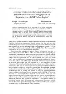
Here we focus on estimating the surface normal nij for each point pij at a given observation vt . In order to do that we consider the 4 or 8 neighbors of the points in the observation matrix [vij ], that is, we are exploiting the 2D layout of the points (see Figure 1). In order to improve robustness, instead of consider each neighboring point, we consider neighboring regions of size l. For each region Ri we take its centroid ri . Then, given the considered point pij and the centroids {r1 , r2 , . . . , rn } of the n neighboring regions we build the vectors αi = ri − pij . Then, the normal nij results from multiplying adjacent vectors in counterclockwise sense and taking the average: nij = ((αn × αn−1 ) + (αn−1 × αn−2 ) + . . . + (α1 × αn ))/n

(1)

As the quality of the latter estimation depends on the number of valid 3D points inside a given region, we consider that the resulting normal is undefined when there is not enough information to provide a robust estimate.

Fig. 1. Estimating the normal at a point using 8 regions: Neighboring regions of size 5 × 5 (left), centroid for each region and associated vector (center), normal vector resulting for applying Expression 1.(right)

4 4.1

Vertical Planes Estimation Removing horizontal planes

Assuming that the floor is flat and also that the height of the camera is constant, and considering the fact that the floor and ceiling planes are usually low textured and in this case their associated stereo points are typically very noisy, we remove these latter planes and we focus on the vertical ones (walls) (see Figure 2).

Fig. 2. Removing the floor and the ceiling. Complete scene with those planes (left). Resulting scene after removing the planes (right).

Once we have only vertical planes, the problem of estimating these planes can be posed in terms of finding in 2D the segments resulting from their projections on the imaginary horizontal plane. In order to do that, we will build a Gaussian Mixture Model classifier for 2D normals where each class is given by the set of points with similar normals (associated to parallel walls). Next, we build the planes associated to each class with a connected-components process. 4.2

Gaussian Mixture Model Classifier

Our one-dimensional mixtures-of-Gaussians classifier [11] is built on a set of n samples X = {x1 , x2 , . . . , xn } that we want to fit with k Gaussian kernels

with unknown parameters {(µ1 , σ1 ), (µ2 , σ2 ), . . . , (µk , σk )}. We must estimate the parameters that maximize the log-likelihood function: ` = log

n X k Y

πj P (xi |j) =

i=1 j=1

n X

log

i=1

k X

πj P (xi |j)

(2)

j=1

where πj is the prior probability of belonging to the kernel j and P (xi |j) is the probability for xi of a Gaussian centered on the kernel j. In order to find the prior probabilities and the parameters of the kernels we apply the standard EM (Expectation-Maximization) algorithm [7]. In the E-step (Expectation) we update the posterior P (j|xi ), that is, the probability that a pattern xi is generated by kernel j: P (j|xi ) = πj P (xj |j)/

k X

πl P (xi |l)

(3)

l=1

In the M-step (Maximization) we proceed to update the priors and the parameters of the kernels given the posteriors computed in the E-step: Pn πj =

i=1

Pn Pn P (j|xi ) P (j|xi )xi 2 P (j|xi )(xi − µj )2 i=1P , µj = Pi=1 , σ = n n j n i=1 P (j|xi ) i=1 P (j|xi )

(4)

Alternating E and M steps the algorithm converges to the closest local maxima with respect to the initialization point. Then, we take the MAP estimate for each normal: M AP (xi ) = arg maxj P (j|xi ), where P (j|xi ) = πj P (xi |j)/P (xi ). 4.3

Classifying normals

In order to classify each normal, we take the relative angle between the reference vector (1,0,0) in the XZ plane. In Figure 3 we represent an example of clasification with real data. We represent the original point cloud with the normal of each point, and the directional histogram with four peaks associated to the four types of parallel planes. Also, we show how are classified the points of the scene. We have used k = 4 kernels whose averages have been randomly initialized from the interval [0, 360]. When the number of kernels is under 4 (for instance we may have only two classes when the robot is in the middle of a corridor), the algorithm also converges because in this case the prior probabilities of the non-existent classes tend to zero. We illustrate this case in Figure 4. Finally, we also consider the pre-filtering of noisy patterns (normals, in this case) in order to avoid distortions in the final result. 4.4

Fitting Vertical Planes

Once we have found the k clases C = {c1 , c2 , . . . , ck } associated to the types of wall appearing in the scene, each cj contains a set of points {pji } with similar normals. Next, we proceed to divide these sets in different vertical planes.

Fig. 3. Classification example using EM algorithm. 2D point cloud for a given scene and their normals (left). Directional histogram and final kernels (center). Final Kernels distributions (right).

Fig. 4. Initial classification of the scene in Figure 2. Normals (left) and final position of the 4 kernels. The prior probabilities are 0.0, 0.42, 0.0 and 0.58 respectively.

Given two points pja and pjb of class cj we consider that they belong to the same plane when the distance between them in the XZ plane is below a given threshold λ: ||pja − pjb ||xz < λ. Given this binary relation we build a graph Gj (V, A) whose vertices are associated to points in the class and the edges are associated to pairs of vertices that satisfy the previous binary relation. Then we calculate the connected components of this graph which represent the vertical planes. Once we have computed the connected components we must estimate the parameters of the vertical planes and their bounds. We consider the set of points with their normals {(p1 , n1 ), (p2 , n2 ), . . . , (pl , nl )} that define a given plane ψ. We take as point and normal of the plane the centroid and the average normal, respectively: ψ = (p, n). The plane’s bounds are obtained by computing the orthogonal plane ψ ⊥ = (p, n⊥ ), and these bounds are determined by the most distant points from this orthogonal plane (see Figure 5). Finally, to consider a plane valid, is necessary to verify that it is sufficiently long and it contains enough points. Once we have computed the vertical planes in 2D, we must to apply their height in 3D, using the floor and ceiling heights (see Figure 6). In the other hand, the vertical planes bounds (floor and ceiling) are calculated using the bounding-box of the vertical planes set.

Fig. 5. Determining the parameters (point, normal and bounds) of each plane.

Fig. 6. Planes detected from the example of the figure 3. Vertical planes in 2D (left) and corresponding 3D planes with horizontal planes also. The algorithm detects 8 vertical planes.

5

Plane texturization

Once we have found the horizontal and vertical planes, we must texturize them using the appearance information of the observations (reference images). Each plane defines a rectangular region of the space which can be parametrically crossed in two directions, horizontal (α) and vertical (β). Each 3D point pαβ of the plane, can be observed by anyone of the t observations {v1 , v2 , . . . , vt }, which we know its respective poses {ϕ1 , ϕ2 , . . . , ϕt }. Using the fundamental matrix of the camera, we project the point on each image. Then, we consult the pixel color in each image, obtaining a set of color candidates for this point {c1 , c2 , . . . , ct }. We must reject the points of this set that are not visible (because there is a vertical plane between the projection and the 3D point). The final color of the point is calculated like closest to the average of the set: arg minci |ci − c¯|. The method is able to obtain a quite realistic texture. Nevertheless, an inherent problem resides in the objects in the scene that do not adjust to any plane. We have observed a smooth effect in this objects when they are captured from different points of view (see experiments section)

6

Experiments and validation

In this section, we present a complete experiment in which we have estimated the planes in a real scene. The scene is composed by 68 observations, along an indoor environment located in the facilities of our department. The original point cloud present 2.025.666 points in 3D (Figure 7 left).

Fig. 7. Original point cloud of the experiment (left). Points and normals after horizontal planes removal (top right). Vertical planes detected (Bottom right).

Using the proposed algorithm, we obtain 11 vertical planes (Figure 7 Bottom right). Its corresponding textures, as well as those of ceiling and ground, have been stored in different images. The complete scene (geometric information of the planes and its corresponding textures) occupies 980 Kb of disk space. Comparatively, the original point cloud mentioned previously occupies 31.652 Kb of disk space. In Figure 8 we show several 3D views of the textured model.

Fig. 8. Several 3D views of the final 3D scene.

7

Conclusions and future work

In this work, we present an algorithm to estimate the principal 3D planes of a scene composed by a set of stereo observations. We have proposed a two-step point classifier based on the normal and the relative positions of the points. Finally, we present an algorithm to estimate the texture of each plane using appearance information of the observations. We are currently investigating in the construction of non-plane primitives from these planes. Our initial idea is, after estimating planes, we model each one with a free approximation surface. Using this technique, we can obtain more realistic scenes. On the other hand, we are interested in detecting other basic primitives like cylinders and spheres.

References 1. S. Thrun et al. “Probabilistic Algorithms and the interactive museum tour-guide robot Minerva”. International Journal of Robotics Research Vol 19 No 11. November 2000. 2. F.Dieter, W. Burgard, S. Thrun “The dynamic window approach to collision avoidance”. IEEE Robotics and Automation Magazine, 1997 3. H.P. Moravec. “Robot spatial perception by stereoscopic vision and 3D evidence grids”. TR The Robotics Institute Carnegie Mellon University. Pittsburgh, Pennsylvania, 1996. 4. S. Se, D. Lowe, J. Little.“Vision-based mobile robot localization and mapping using scale-invariant features” Proc. of IEEE International Conference on Robotics and Automation. Seoul, Korea May 2001. 5. L. Iocchi, K. Konolige, M. Bajracharya. “Visually realistic mapping of planar environment with stereo”. Seventh International Symposium on Experimental Robotics (ISER’2000). Hawaii 2000. 6. Y. Liu, R. Emery, D. Chakrabarti, W. Burgard, S. Thrun. “Using EM to learn 3D models of indoor enviroments with mobile robots”. Eighteenth International Conference on Machine Learning. Williams College, June 2001. 7. A. Dempster, A. Laird, D. Rubin. “Maximum likelihood from incomplete data via the EM algorithm”. Journal of the Royal Statistical Society, Series B 39, 1 38. 1977 8. I. Stamos, M. Leordeanu. “Automated Feature-Based Range Registration of Urban Scenes of Large Scale”. IEEE International Conference of Computer Vision and Pattern Recognition, pp. 555-561, Vol. II, Madison, WI, 2003. 9. J.M. S´ aez, F. Escolano “Monte Carlo Localization in 3D Maps Using Stereo Vision”. In: Garijo, F.J., Riquelme, J.C., Toro, M.(eds.): Advances in Artificial Intelligence - Iberamia 2002. Lecture Notes in Computer Science, Vol. 2527. Springer-Verlag, Berlin Heidelberg New York (2002) 913-922. 10. J.M. S´ aez, A. Pe˜ nalver, F. Escolano “Estimaci´ on de las acciones de un robot utilizando visi´ on est´ereo”. IV Workshop de Agentes F´ısicos (WAF 2003). Alicante, Abril de 2003. 11. R.A. Redner, H.F. Walker. “Mixture Densities, Maximum Likelihood, and the EM Algorithm”. SIAM Review, 26(2):195-239, 1984.