Remembrance of Transistors Past: Compact Model Parameter Extraction Using Bayesian Inference and Incomplete New Measurements Li Yu, Sharad Saxena1 , Christopher Hess1 , Abe Elfadel2 , Dimitri Antoniadis, Duane Boning Massachusetts Institute of Technology, 1 PDF Solutions, 2 Masdar Institute of Science and Technology Email:
[email protected] ABSTRACT In this paper, we propose a novel MOSFET parameter extraction method to enable early technology evaluation. The distinguishing feature of the proposed method is that it enables the extraction of an entire set of MOSFET model parameters using limited and incomplete IV measurements from on-chip monitor circuits. An important step in this method is the use of maximum-a-posteriori estimation where past measurements of transistors from various technologies are used to learn a prior distribution and its uncertainty matrix for the parameters of the target technology. The framework then utilizes Bayesian inference to facilitate extraction using a very small set of additional measurements. The proposed method is validated using various past technologies and post-silicon measurements for a commercial 28-nm process. The proposed extraction could also be used to characterize the statistical variations of MOSFETs with the significant benefit that some constraints required by the backward propagation of variance (BPV) method are relaxed.
Keywords MIT Virtual Source (MVS) MOSFET model, parameter extraction, Bayesian inference, maximum-a-posteriori (MAP) estimation
1.
INTRODUCTION
Continued scaling of CMOS technology has introduced new physical mechanisms for short-channel devices which significantly increase the number of parameters and the complexity of equations of a compact transistor model. To be effectively used in circuit design simulations, all the many dozens of model parameters need to be carefully extracted from multiple test structures (e.g., I-V structures, C-V structures, ring oscillators, etc) so that the model can accurately reproduce the transistor electrical characteristics. Usually the set of model parameters is divided into subsets of local and global parameters, where the local parameters apply to a single device dimension while global parameters apply to all relevant device geometries [1]. Therefore experimental data for devices with different geometries and replicas are needed to find the global set of parameters. The most widely used parameter extraction methods are based on the deterministic minimization of an error function between model output and measurement data. Algorithms used to solve the optimization problem are either gradient-based (e.g., Levenberg-Marquardt) or gradient-free (e.g., Genetic Algorithm - GA). GA mimics the natural selection and evolution process and is more likely to find the global minimum [2]. All these minimization methods are iterative, and defining an appropriate starting point and parameter bounds is of crucial importance and requires considerable experience. Furthermore, for a given set of measurements, there may be multiple minimizing solutions, and selecting the one most compatible with the physics of the device is a difficult task. Permission to make digital or hard copies of all or part of this work for personal or classroom use is granted without fee provided that copies are not made or distributed for profit or commercial advantage and that copies bear this notice and the full citation on the first page. Copyrights for components of this work owned by others than ACM must be honored. Abstracting with credit is permitted. To copy otherwise, or republish, to post on servers or to redistribute to lists, requires prior specific permission and/or a fee. DAC ’14, June 01 - 05 2014, San Francisco, CA, USA Copyright 2014 ACM 978-1-4503-2730-5/14/06$15.00. http://dx.doi.org/10.1145/2593069.2593201
The situation becomes even worse in the presence of significant measurement “noise” which introduces unavoidable errors in the extracted model parameter, thus compromising even further their physical significance. Traditional silicon characterization and extraction flows suffer from 1) large area overhead due to the complexity of different test structures and transistor geometries; and 2) long testing time due to a very limited number of I/O ports through which all measurement data for all test structures have to be collected. This problem is further exacerbated in statistical parameter extraction which is used in statistical IC analysis and optimization, e.g., statistical static timing analysis and post-silicon tuning. In nanoscale technologies, IC testing has contributed to a significant portion of the total manufacturing cost to the point that it is now almost impossible to cover all I-V measurements for every on-chip monitoring device on each die in a wafer. Existing statistical parameter extraction methods such as the backward propagation of variance (BPV) [3][4] are advantageous only when the number of measurements is larger than the number of model parameters. They also impose the stringent constraint that extracted parameters must be statistically uncorrelated. Such limitations mean, among several similar situations, that the correlated variations in sub-threshold swing (SS) and threshold voltage (Vth0 ) cannot be extracted at the same time. In this work, we exploit recent advances in statistics and semiconductor metrology to develop a novel and unified MOSFETs parameter extraction method for low-cost silicon testing and characterization. While the virtual probe described in [5] and in [6] focus on reducing the number of measured dies needed to characterize spatial variation, our work focuses on reducing testing cost per die. Our new method is general, allows for the absence of I-V measurements in the data set, removes the independence restriction on the model parameters and could be used to conduct both deterministic and statistical model parameter extraction. While our theory and algorithms are independent of the underlying transistor model (BSIM, PSP, EKV, MVS, etc.), we mainly use the MIT Virtual Source (MVS) model to illustrate the applicability of our work to deeply-scaled devices where the main mode of charge transport is quasiballistic. The intrinsic simplicity of the MVS model combined with the Bayesian inference [7] framework enables the statistical extraction of an entire parameter set using only 6 noisy I-V measurements. A key step in this new method is the maximum-a-posteriori (MAP) estimation where past I-V measurements of older transistor technologies are used and learned to obtain a prior distribution on the parameter set along with its uncertainty matrix.
2.
MVS MODEL AND PARAMETERS
The MIT virtual source (MVS) model is an ultra compact, charge-based MOSFET model that provides a simple, physics-based description of carrier transport in modern short-channel MOSFET [8] [9][10]. It essentially substitutes the quasi-ballistic carrier transport concept for the concept of drift-diffusion with velocity saturation. In doing so, it achieves excellent accuracy for the I-V and C-V characteristics with continuity of current and its derivatives throughout all regions of operation. The VS model has the advantage of using a limited number of input parameters, most of which have straightforward physical meanings and can be easily measured using traditional device characterization.
Fig. 1 shows the parameter extraction methodology for MVS with the key parameters extracted from I-V measurements highlighted. Table 1 summarizes these key parameters along with their physical meaning.
Similarly, we assume that the above-threshold current Fn follows a Gaussian distribution: ) Fn ∼ N (f (Vn , Psub , Pabove ), βF−1 n
(2)
where βF−1 is the precision (inverse variance) for Fn . n The least-squares error function of sub-threshold and above-threshold regions are, respectively, E(Psub ) =
N 1 X {ln(Fn ) − ln(f (Vn , Psub , Pabove ))}2 2 n=1
E(Pabove ) =
N 1 X {Fn − f (Vn , Psub , Pabove )}2 2 n=1
(3)
(4)
In the next section, we present a maximum-a-posteriori (MAP) estimation of Pabove and Psub where instead of minimizing the error function in (3) and (4), we will maximize the probability of observing F.
3. MAXIMUM A POSTERIORI ESTIMATION 3.1 Physical Subspace Projection
Figure 1: Optimization flow for I-V parameter extraction in the MVS model.
Table 1: Key parameters extracted with experimental data for the MVS model with physical meaning. Parameters Description V t0(V ) Strong inversion threshold voltage n0 Sub-threshold swing factor δ(mV /V ) Drain-induced barrier lowering vxo (cm/s) Virtual source carrier velocity µ(cm2 /V · s) Low-field mobility Rs0(ohm · µm) Series resistance per side The extracted parameters are divided into two groups: one for the sub-threshold region (V t0, n0 and δ) and one for the above-threshold region (vxo , µ, Rs0, etc.). In traditional device characterization, each group is optimized separately using non-linear least-squares error minimization [11].
2.1
To formalize the parameter extraction problem, we consider a measurement set of currents {F1 , ..., FN } with corresponding inputs V = {V1 , ..., VN }. We group the target variables {Fn } into a vector that we denote by F. Each input contains voltages from four terminals Vn = {Vgn , Vdn , Vsn , Vbn }. We define Psub = {V t0, n0, δ} as the sub-threshold parameters and Pabove = {vxo , µ, Rs0, ...} as the above-threshold region parameters. We call the submanifolds of Psub and Pabove the physical subspace since each is a multidimensional surface parameterized with the physical parameters in the MVS model. The output of the MVS model would then be f (V, Psub , Pabove ). The problem we aim to address is to estimate Psub and Pabove given the observations {F1 , ..., FN } with the challenge that the size of the measurement set N is very small. Based on the physics of transistor operation in the subthreshold regime, we assume that the measurement of subthreshold currents Fn follows a log-normal distribution:
−1 where βlnF is the precision (inverse variance) of lnFn . n
Without loss of generality, we describe the MAP estimation for sub-threshold parameters. Above-threshold parameters could be estimated in a similar manner. First, we assume that Psub follows a Gaussian distribution Psub ∼ N (µPsub , ΣPsub ): pdf (Psub ) = q
1 (2π)ksub ΣPsub
1 ·exp[− (µPsub − Psub )T Σ−1 Psub (µPsub − Psub )] 2
(1)
(5)
where µPsub and ΣPsub are the mean vector and covariance matrix of the sub-threshold region parameters, respectively, and where ksub is the dimension of Psub . Next, we assume that the “uncertainty” of µPsub follows a conjugate Gaussian prior distribution µPsub ∼ N (µs0 , Σs0 ). pdf (µPsub ) = p
Problem Definition
−1 lnFn ∼ N (lnf (Vn , Psub , Pabove ), βlnF ) n
The purpose of physical subspace projection is to relate an observed measurement to an output of the physics-based model and use both to derive a probability distribution on the physical subspace [12]. In the transistor model extraction context, it means to relate current measurements at different voltage biases to the outputs in the sub-threshold and above-threshold physical subspace Psub and Pabove , respectively. The pdf ’s on Psub or Pabove can then be calculated and the parameter extraction problem solved using maximum a posteriori (MAP) estimation.
1
(2π)k |Σs0 | 1 ·exp[− (µPsub − µs0 )T Σ−1 s0 (µPsub − µs0 )] 2
(6)
where µs0 and Σs0 are the mean vector and covariance matrix of µPsub , respectively. Given µPsub and βlnFn , we calculate the probability of observing each data point lnFn associated with subspace distribution pdf (Psub ) as r
βlnFn 2π (lnFn − lnf (Vn , µPsub , µPabove ))2
pdf (lnFn |µPsub , βlnFn ) = ·exp[−
2·
−1 βlnF n
(7) ]
The above equation (7) is the complete form of the physical subspace projection for the sub-threshold region.
3.2
Learning Precision at Different Biases
The learning of precision βlnFn is a key step in physical subspace projection. In practice, many reasons may contribute to the uncertainties of measurements at each bias. These reasons include modeling errors due to the inability of MVS to capture certain physical effects or measurment
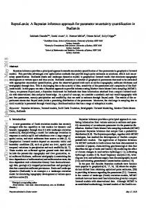
errors due to inaccuracies in current measurements. While they depend on the details of the fabrication or measurement process, these uncertainties show a strong systematic trend at different bias. In this work, the IV curves of transistors from past technologies or past transistor data from current technologies are used to learn the systematic MVS model uncertainty trend at different voltage biases. Such data may come from either test-site measurement or simulations using mature or early product design kits. The detailed learning process proceeds as follows. First, a group of historical transistors are selected depending on the fabrication process of the target transistor. For example, if we intend to fit a transistor fabricated in a low power process, appropriate historical transistors would also be transistors in a low power process. Since no detailed information about the target transistor is available, a mix of short-channel transistors in several fabrication processes and technology nodes (six in this paper) are employed to improve our confidence in predicting βlnFn on an unknown transistor. This assumes that although a new process introduces different lithography, structures and materials, the basic function transistors operate do not change. Therefore the MVS parameters do not drastically change because most of them are from direct measurements rather than fabrication process. After selection of a group of historical transistors, each selected transistor is fitted into the MVS model with a complete set of IV measurements using the deterministic, non-linear, least-squares (NLS) error q function, Equations (3) −1 is calculated by the and (4). The standard deviation βlnF n average differences between measurements and MVS model predictions using the NLS extracted parameters. q −1 ) at Fig. 2 shows a learned standard deviation ( βlnF n different voltage biases. Fig. 2 (a) shows an extraction of average uncertainty from design kits when a clean data set with no measurement error is involved. A high uncertainty is observed on Idsat with very low gate voltage because the MVS model is an ultra-compact model that is unable to capture the gate tunneling effect. Fig. 2 (b) shows an extraction of average uncertainty from measurement data where the uncertainty includes both modeling and measurement errors. A rapid increase of uncertainty is observed on Idlin at very low gate voltage region. This is due to the inaccuracies of current measurement in the sub-nA region. Similarly, Fig. 3
q Figure 3: Extraction of average uncertainty βF−1 n at different biases for 6 different technologies from measurement results. µPsub and βlnFn . We then combine this conditional probability with the prior distribution pdf (µPsub ) in (6) to accurately estimate µPsub . Assuming each current measurement is independent, we can write the likelihood function pdf (F|µPsub , βlnFn ) as: N Y
pdf (F|µPsub , βlnFn ) =
pdf (Fn |µPsub , βlnFn )
(8)
n=1
According to Bayes’ theory, the conditional distribution pdf (µPsub |F) is proportional to the product of the prior pdf (µPsub ) and the likelihood function pdf (F|µPsub ): pdf (µPsub |F) ∝ pdf (µPsub ) · pdf (F|µPsub )
(9)
The precision βlnFn is learned from historical transistor data and is therefore independent of the measurement set F. Consequently, pdf (F|µPsub , βlnFn ) = pdf (F|µPsub )
(10)
Substituting (8) and (10) into (9) yields: pdf (µPsub |F) ∝ pdf (µPsub ) ·
N Y
pdf (Fn |µPsub , βlnFn )
(11)
n=1
q −1 Figure 2: Extraction of average uncertainty βlnF n at different bias for 6 different technologies from (a) design kits, and (b) measurement results. q shows an extraction of average uncertainty βF−1 from mean surement data for the above-threshold region. It will be used to extract Pabove .
3.3
Learning a Prior Distribution
After physical subspace projection and precision estimation, we are able to project very small samples in current measurements {F1 , ..., FN } to parameter subspace Psub and obtain the conditional probability of observing lnFn given
The above equation demonstrates the sequential nature of Bayesian learning in which the “old” posterior distribution becomes the “new” prior when a new data point is added to the measurement set. Fig. 4 shows the results of Bayesian learning on µPsub as the portfolio of the measurement groups is expanded. We only show a 2-D map of delta and SS (sub-threshold swing which is the physical expression of n0). The third sub-threshold parameter Vt0 is fixed for better comparisons across all measurement updates. The bottom left figure corresponds to the situation before any data points are observed and shows a plot of the prior distribution µPsub ∼ N (µs0 , Σs0 ). Note that µs0 and Σs0 are learned from historical transistor data in exactly the same way as βlnFn . A complete set of IV measurements for short-channel transistors with 6 different fabrication processes and technology nodes are fitted into the MVS model using the leastsquares error functions, giving us the a priori µs0 and Σs0 MVS model parameters. We then derive the mean and standard deviation of transistor currents at each bias voltage using µs0 and Σs0 . Fig. 5 shows the mean and standard deviation of the transistor IV curves using the extracted µs0 and Σs0 ; these provide the prior distributions before collecting any new measurements for the target technology. Notice that
Figure 4: Illustration of sequential Bayesian learning of µPsub using priors and IV measurements. The two parameters shown are the sub-threshold swing factor SS and the drain-induced barrier lowering δ. The red color represents estimates with high likelihood while the blue color represents estimates with low likelihood. As more measurements are added, the MAP parameter estimates become more accurate. constant items yield: E(Psub ) = +
1 (µ − µs0 )T Σ−1 s0 (µPsub − µs0 ) 2 Psub
N 1 X βlnFn {ln(Fn ) − ln(f (Vn , Psub , Pabove ))}2 2 n=1
(12)
Similarly, we have E(Pabove ) =
1 (µ − µf 0 )T Σ−1 f 0 (µPabove − µf 0 ) 2 Pabove N 1 X + βF {Fn − f (Vn , Psub , Pabove )}2 2 n=1 n (13)
Figure 5: Mean and standard deviation of the transistor IV curve using µs0 and Σs0 learned from historical transistor data. The first row of Fig. 4 shows the resulting likelihood function pdf (Fn |µPsub ) for measurements at different biases alone. Different widths of red regions at each bias represents historical learning of βlnFn . If two measurements have large discrepancy (e.g. SS from the first and third samples), the extraction results will be more strongly adjusted toward the measurement with the higher precision (narrower width). The second row shows the posterior distribution pdf (µPsub |F) which results from multiplying its likelihood function from the top row by the prior (bottom left). As this process continues, the posterior distribution becomes much sharper, and in the limit of an infinite number of data points, the posterior distribution would become a delta function centered on the true parameter values.
3.4
Maximum-A-Posteriori Estimation
Our final goal is to find optimal estimates of µPsub and µPabove that maximize the log likelihood of the posterior distributions lnpdf (µPsub |F) and lnpdf (µPabove |F), respectively. Substituting (6) and (7) into (11) and removing the
Equations (12) and (13) are the new error functions given by maximum-a-posteriori (MAP) estimation. Compared with (3) and (4), we note the following two advantages: 1) a biasdependent precision allocating weights to sample measurement errors as contrasted with the uniform weights of NLS; 2) an appropriate prior distribution that has been learned from historical transistor data and which provides a parameter probability distribution before any measurement. In particular, the BPV restriction that the number of electrical measurements should be larger than the number of extracted parameters is removed.
4.
VALIDATION
In this section, two model parameter extraction examples in several cutting-edge CMOS technologies are used to demonstrate the efficiency of our method. To test and compare with the prior art, we have also implemented deterministic extraction using the non-linear least-squares error function and statistical extraction using backward propagation of variance (BPV).
4.1
Example I: Early Technology Evaluation
The first example is to use the MVS model for early technology evaluation. The difficulty of this problem is that measurements are collected from a limited number of early prototype devices rather than from a full suite of designed test structures. Therefore it is highly unlikely that the limited data will be sufficient to fit complex compact models such as BSIM. As for the ultra compact MVS model, separate measurements of Id − Vds and Id − Vgs are needed in
order to apply the traditional deterministic method of nonlinear least squares error function. Fig. 6 shows the MVS model fitting results using our new parameter extraction method for 4 technologies from 14nm through 45nm. Notice that some technologies are not used for learning the prior information and only 6 points from Id − Vgs are used to fit the entire model. The prediction results on the rest of measurements match well throughout the operating region, including the Id − Vds curves. Even for transistors with gate tunneling effects (e.g., technology 3), the proposed method would still extracts the correct trend in the sub-threshold region. This is because according to the historical record, the MVS model may suffer a large modeling error in this region and therefore less weight would be assigned for the Iof f measurement. Fig. 7 shows an average MVS model prediction error for technology 3 using both our MAP method and the least-squares error function. A 3X sample size reduction is observed.
example where we focus on characterizing a target transistor, here we emphasize modeling statistical distribution of groups of transistors and trying extract to distribution of their MVS parameters. The bottleneck here is that in order to obtain a statistically sufficient number of transistors, we suffer from the testing costs from tens of thousands of transistors. To extract key parameters (e.g., Idsat , Idlin , Vtsat and Vtlin ) and save testing costs, typically only a small set of IV curve data is collected. In a standard BSIM model, these few IV measurements are not sufficient to extract all parameters. Some knowledge of, or restrictions on, many of the BSIM parameters is needed. On the other hand, Fig. 8 shows MVS model fitting with two transistor measurements in a 28nm technology using our MAP parameter extraction method. Only 6 measurements are used to fit 8 parameters in the MVS model, and the prediction matches well with other test measurements.
Figure 8: MVS model fitting results using the MAP parameter extraction method in a 28-nm technology from wafer measurements. The blue circles are fitting measurements used by the proposed method. The red circles are additional test measurements used for validation.
Figure 6: MVS model fitting results using MAP parameter extraction method in 4 technologies in 14nm-45nm. Blue circles are fitted measurements using the MAP method and red circles are test measurements for validation.
This suggests an alternative method for extracting variations of VS model parameters from wafer level measurements. The method consists in simply extracting deterministic MVS parameters separately for many devices and calculating their covariance matrix. Compared with the traditional BPV method, this direct method has several advantages. First, the relationship between measurements at different bias is maintained. For example, the extraction of sub-threshold swing SS needs measurements at more than two biases in the sub-threshold region and therefore it is hard to extract its variance through BPV. Second, BPV assumes independent parameters, and correlated variables cannot be extracted with the same backward propagation. Third, BPV requires the number of electrical measurements to be larger that the number of extracted parameters, which in turn requires a significant number of measurements, especially for complex compact models such as BSIM and PSP. In contrast, this direct statistical extraction is more accurate and is less constrained. Fig. 9 shows Id probability density simulated using variance extracted through our MAP method compared with variance extracted using BPV, together with measurements at two different biases. Both methods show an accurate distribution for Idsat but the MAP method shows a much better prediction for Id current distribution in the transition region (Vd = Vdd , Vg = Vdd /2).
Figure 7: Average model prediction error for technology 3 on Id for above-threshold region and log10 Id for the sub-threshold region, showing reduced error of proposed method compared to traditional NLS method.
4.2
Example II: Statistical Extraction for postSilicon Validation
The second example is to use the MVS model to estimate post-Silicon circuit performance or to conduct statistical parameter extraction. In both cases, measurements are taken from different on-chip monitor circuits in which a large number of transistors is involved. Unlike the first
Figure 9: Id probability density simulated using variance extracted through proposed method compared with variance extracted through BPV, together with measurements at two different biases. Fig. 10 shows statistically-extracted wafer maps of key MVS model parameters V t0, delta, SS, vxo and µ in a 28-
nm technology. A strong correlation is observed between vxo and µ, which matches the theoretical prediction given by [13] that the relative change in virtual source velocity is proportional to the change in mobility. Fig. 11 shows a scatter plot of virtual source velocity and mobility from extraction of on-chip monitor circuits of one 28nm wafer. We observe that 83% of the relative change in mobility is converted to relative change in virtual source velocity, which is very close to 85% given by [13]. This shows that the proposed method is able to correctly extract and separate strongly correlated parameters even with very limited measurements.
the joint statistics of the parameters, and the biasing of the devices.
Acknowledgment The themes and title of this work were inspired by Liu et al. [14]. This work was funded by the Cooperative Agreement Between the Masdar Institute of Science and Technology, Abu Dhabi, UAE and the Massachusetts Institute of Technology, Cambridge, MA, USA, Reference 196F/002/ 707/102f/70/9374.
References
[1] S. Yao, T.H. Morshed, D.D. Lu, S. Venugopalan, W. Xiong, C.R. Cleavelin, A.M. Niknejad, and C. Hu. Global parameter extraction for a multi-gate MOSFETs compact model. In IEEE International Conference on Microelectronic Test Structures (ICMTS), pages 194–197, 2010. [2] Q. Zhou, W. Yao, W. Wu, X. Li, Z. Zhu, and G. Gildenblat. Parameter extraction for the PSP MOSFET model by the combination of genetic and Levenberg-Marquardt algorithms. In IEEE International Conference on Microelectronic Test Structures (ICMTS), pages 137–142, 2009. [3] C.C. Mcandrew, Xin Li, I. Stevanovic, and G. Gildenblat. Extensions to backward propagation of variance for statistical modeling. IEEE Design Test of Computers, 27(2):36–43, 2010. [4] L. Yu, L. Wei, D. Antoniadis, I. Elfadel, and D. Boning. Statistical modeling with the virtual source mosfet model. In Design, Automation Test in Europe Conference Exhibition (DATE), 2013, pages 1454–1457, March 2013.
Figure 10: Statistically-extracted wafer maps of key VS model parameters V t0, delta, SS, vxo and µ in a 28-nm technology. Parameter correlations are also shown in the bottom right table.
[5] W. Zhang, X. Li, T. Liu, E. Acar, R.A. Rutenbar, and R.D. Blanton. Virtual probe: A statistical framework for lowcost silicon characterization of nanoscale integrated circuits. IEEE Transactions on Computer-Aided Design of Integrated Circuits and Systems, 30(12):1814–1827, 2011. [6] S. Reda and S.R. Nassif. Analyzing the impact of process variations on parametric measurements: Novel models and applications. In Design, Automation Test in Europe (DATE), pages 375–380, April 2009. [7] C. M. Bishop. Pattern Recognition and Machine Learning. Springer-Verlag New York, Inc., Secaucus, NJ, USA, 2006. [8] S. Rakheja and D. Antoniadis. MVS 1.0.1 nanotransistor model (silicon), Nov 2013. [9] A. Khakifirooz, O.M. Nayfeh, and D. Antoniadis. A simple semiempirical short-channel MOSFET current-voltage model continuous across all regions of operation and employing only physical parameters. IEEE Transactions on Electron Devices, 56(8):1674 – 1680, Aug. 2009.
Figure 11: Scatter plot for statistically extracted virtual source velocity and mobility from on-chip monitor circuits of one wafer from a 28nm technology.
5. CONCLUSION In this paper, we propose a novel MOSFET parameter extraction method using maximum-a-posteriori (MAP) estimation, which successfully extracts an entire set of MOSFET model parameters using limited and incomplete IV measurements from on-chip monitor circuits. The key idea in this work is to exploit the fact that model parameters of a unknown transistor are correlated with model parameters of existing historical transistors. The framework adopts a Bayesian inference approach to facilitate the extraction procedure. Historical knowledge of transistor performances is learned from various technologies as a priori information, where the learning is achieved by performing extraction on complete IV curves through traditional non-linear least square error functions. Maximum-a-posteriori estimation is then applied using the prior. The uncertainty matrix is determined by both transistor model accuracy and measurement error at each voltage bias. The proposed method is validated by various technologies and post-silicon measurements for a commercial 28-nm process. The proposed MAP extraction could also be used to characterize the statistical variations of MOSFETs. The advantage of the MAP method is that it removes the constraints imposed by the backward propagation of variance on large number of measurements,
[10] L. Wei, O. Mysore, and D. Antoniadis. Virtual-source-based self-consistent current and charge FET models: From ballistic to drift-diffusion velocity-saturation operation. IEEE Transactions on Electron Devices, (99):1 – 9, 2012. [11] L. Yu, O. Mysore, L. Wei, L. Daniel, D. Antoniadis, I. Elfadel, and D. Boning. An ultra-compact virtual source fet model for deeply-scaled devices: Parameter extraction and validation for standard cell libraries and digital circuits. In Asia and South Pacific Design Automation Conference(ASPDAC), pages 521–526, 2013. [12] L. Yu, S. Saxena, C. Hess, I. Elfadel, D. Antoniadis, and D. Boning. Efficient performance estimation with very small sample size via physical subspace projection and maximum a posteriori estimation. In Design, Automation and Test in Europe (DATE), 2014. [13] A. Khakifirooz and D.A. Antoniadis. Transistor performance scaling: The role of virtual source velocity and its mobility dependence. In International Electron Devices Meeting (IEDM), Dec. 2006. [14] H Liu, A. Singhee, R.A. Rutenbar, and L.R. Carley. Remembrance of circuits past: macromodeling by data mining in large analog design spaces. In Design Automation Conference (DAC), pages 437–442, 2002.