(Automated Similarity Judgment Program) project2 represents such an approach, where ... 2 http://email.eva.mpg.de/~wichmann/ASJPHomePage.htm. 3 At this ...
Comparative evaluation of string similarity measures for automatic language classification. Taraka Rama and Lars Borin
1 Introduction Historical linguistics, the oldest branch of modern linguistics, deals with language-relatedness and language change across space and time. Historical linguists apply the widely-tested comparative method [Durie and Ross, 1996] to establish relationships between languages to posit a language family and to reconstruct the proto-language for a language family. 1 Although historical linguistics has parallel origins with biology [Atkinson and Gray, 2005], unlike the biologists, mainstream historical linguists have seldom been enthusiastic about using quantitative methods for the discovery of language relationships or investigating the structure of a language family, except for Kroeber and Chrétien [1937] and Ellegård [1959]. A short period of enthusiastic application of quantitative methods initiated by Swadesh [1950] ended with the heavy criticism levelled against it by Bergsland and Vogt [1962]. The field of computational historical linguistics did not receive much attention again until the beginning of the 1990s, with the exception of two noteworthy doctoral dissertations, by Sankoff [1969] and Embleton [1986]. In traditional lexicostatistics, as introduced by Swadesh [1952], distances between languages are based on human expert cognacy judgments of items in standardized word lists, e.g., the Swadesh lists [Swadesh, 1955]. In the terminology of historical linguistics, cognates are related words across languages that can be traced directly back to the proto-language. Cognates are identified through regular sound correspondences. Sometimes cognates have similar surface form and related meanings. Examples of such revealing kind of cognates are: English ∼ German night ∼ Nacht ‘night’ and hound ∼ Hund ‘dog’. If a word has undergone many changes then the relatedness is not obvious from visual inspection and one needs to look into the history of the word to exactly understand the sound changes which resulted in the synchronic form. For instance, the English ∼ Hindi wheel ∼ chakra ‘wheel’ are cognates w
w
and can be traced back to the proto-Indo-European root k ek lo-. 1
The Indo-European family is a classical case of the successful application of comparative method which establishes a tree relationship between some of the most widely spoken languages in the world.
Recently, some researchers have turned to approaches more amenable to automation, hoping that large-scale lexicostatistical language classification will thus become feasible. The ASJP (Automated Similarity Judgment Program) project2 represents such an approach, where automatically estimated distances between languages are provided as input to phylogenetic programs originally developed in computational biology [Felsenstein, 2004], for the purpose of inferring genetic relationships among organisms. As noted above, traditional lexicostatistics assumes that the cognate judgments for a group of languages have been supplied beforehand. Given a standardized word list, consisting of 40–100 items, the distance between a pair of languages is defined as the percentage of shared cognates subtracted from 100%. This procedure is applied to all pairs of languages under consideration, to produce a pairwise inter-language distance matrix. This inter-language distance matrix is then supplied to a tree-building algorithm such as Neighbor-Joining (NJ; Saitou and Nei, 1987) or a clustering algorithm such as Unweighted Pair Group Method with Arithmetic Mean (UPGMA; Sokal and Michener, 1958) to infer a tree structure for the set of languages. Swadesh [1950] applies essentially this method – although completely manually – to the Salishan languages. The resulting “family tree” is reproduced in figure 1. The crucial element in these automated approaches is the method used for determining the overall similarity between two word lists.3 Often, this is some variant of the popular edit distance or Levenshtein distance (LD; Levenshtein, 1966). LD for a pair of strings is defined as the minimum number of symbol (character) additions, deletions and substitutions needed to transform one string into the other. A modified LD (called LDND) is used by the ASJP consortium, as reported in their publications (e.g., Bakker et al. 2009 and Holman et al. 2008).
2 Related Work Cognate identification and tree inference are closely related tasks in historical linguistics. Considering each task as a computational module would mean that each cognate set identified across a set of tentatively related languages feed into the refinement of the tree inferred at each step. In a critical article, Nichols [1996] points out that the historical 2 3
http://email.eva.mpg.de/~wichmann/ASJPHomePage.htm At this point, we use “word list” and “language” interchangeably. Strictly speaking, a language, as identified by its ISO 639-3 code, can have as many word lists as it has recognized (described) varieties, i.e., doculects [Nordhoff and Hammarström, 2011].
linguistics enterprise, since its beginning, always used a refinement procedure to posit relatedness and tree structure for a set of tentatively related languages. 4 The inter-language distance approach to tree-building, is incidentally straightforward and comparably accurate in comparison to the computationally intensive Bayesian-based tree-inference approach of Greenhill and Gray [2009].5 The inter-language distances are either an aggregate score of the pairwise item distances or based on a distributional similarity score. The string similarity measures used for the task of cognate identification can also be used for computing the similarity between two lexical items for a particular word sense. File = salish_swadesh_1.png Figure 1: Salishan language family box-diagram from Swadesh 1950.
2.1 Cognate identification The task of automatic cognate identification has received a lot of attention in language technology. Kondrak [2002a] compares a number of algorithms based on phonetic and orthographical similarity for judging the cognateness of a word pair. His work surveys string similarity/distance measures such as edit distance, dice coefficient, and longest common subsequence ratio (LCSR) for the task of cognate identification. It has to be noted that, until recently [Hauer and Kondrak, 2011, List, 2012], most of the work in cognate identification focused on determining the cognateness between a word pair and not among a set of words sharing the same meaning. Ellison and Kirby [2006] use Scaled Edit Distance (SED) 6 for computing intra-lexical similarity for estimating language distances based on the dataset of Indo-European languages prepared by Dyen et al. [1992]. The language distance matrix is then given as input to the NJ algorithm – as implemented in the PHYLIP package [Felsenstein, 2002] – to infer a tree for 87 Indo-European languages. They make a qualitative evaluation of the inferred tree against the standard Indo-European tree. Kondrak [2000] developed a string matching algorithm based on articulatory features (called 4 This idea is quite similar to the well-known Expectation-Maximization paradigm in machine learning. Kondrak [2002b] employs this paradigm for extracting sound correspondences by pairwise comparisons of word lists for the task of cognate identification. A recent paper by Bouchard-Côté et al. [2013] employs a feed-back procedure for the reconstruction of Proto-Austronesian with a great success. 5 For a comparison of these methods, see Wichmann and Rama, 2014. 6 SED is defined as the edit distance normalized by the average of the lengths of the pair of strings.
ALINE) for computing the similarity between a word pair. ALINE was evaluated for the task of cognate identification against machine learning algorithms such as Dynamic Bayesian Networks and Pairwise HMMs for automatic cognate identification [Kondrak and Sherif, 2006]. Even though the approach is technically sound, it suffers due to the very coarse phonetic transcription used in Dyen et al.’s Indo-European dataset.7 Inkpen et al. [2005] compared various string similarity measures for the task of automatic cognate identification for two closely related languages: English and French. The paper shows an impressive array of string similarity measures. However, the results are very language-specific, and it is not clear that they can be generalized even to the rest of the Indo-European family. Petroni and Serva [2010] use a modified version of Levenshtein distance for inferring the trees of the Indo-European and Austronesian language families. LD is usually normalized by the maximum of the lengths of the two words to account for length bias. The length normalized LD can then be used in computing distances between a pair of word lists in at least two ways: LDN and LDND (Levenshtein Distance Normalized Divided). LDN is computed as the sum of the length normalized Levenshtein distance between the words occupying the same meaning slot divided by the number of word pairs. Similarity between phoneme inventories and chance similarity might cause a pair of not-so related languages to show up as related languages. This is compensated for by computing the length-normalized Levenshtein distance between all the pairs of words occupying different meaning slots and summing the different word-pair distances. The summed Levenshtein distance between the words occupying the same meaning slots is divided by the sum of Levenshtein distances between different meaning slots. The intuition behind this idea is that if two languages are shown to be similar (small distance) due to accidental chance similarity then the denominator would also be small and the ratio would be high. If the languages are not related and also share no accidental chance similarity, then the distance as computed in the numerator would be unaffected by the denominator. If the languages are related then the distance as computed in the numerator is small anyway, whereas the denominator would be large since the languages are similar due to genetic 7
The dataset contains 200-word Swadesh lists for 95 language varieties. Available on http://www. wordgumbo.com/ie/cmp/index.htm.
relationship and not from chance similarity. Hence, the final ratio would be smaller than the original distance given in the numerator. Petroni and Serva [2010] claim that LDN is more suitable than LDND for measuring linguistic distances. In reply, Wichmann et al. [2010a] empirically show that LDND performs better than LDN for distinguishing pairs of languages belonging to the same family from pairs of languages belonging to different families. As noted by Jäger [2014], Levenshtein distance only matches strings based on symbol identity whereas a graded notion of sound similarity would be a closer approximation to historical linguistics as well as achieving better results at the task of phylogenetic inference. Jäger [2014] uses empirically determined weights between symbol pairs (from computational dialectometry; Wieling et al. 2009) to compute distances between ASJP word lists and finds that there is an improvement over LDND at the task of internal classification of languages.
2.2 Distributional similarity measures Huffman [1998] compute pairwise language distances based on character n-grams extracted from Bible texts in European and American Indian languages (mostly from the Mayan language family). Singh and Surana [2007] use character n-grams extracted from raw comparable corpora of ten languages from the Indian subcontinent for computing the pairwise language distances between languages belonging to two different language families (Indo-Aryan and Dravidian). Rama and Singh [2009] introduce a factored language model based on articulatory features to induce an articulatory feature level n-gram model from the dataset of Singh and Surana, 2007. The feature n-grams of each language pair are compared using a distributional similarity measure called cross-entropy to yield a single point distance between the language pair. These scholars find that the distributional distances agree with the standard classification to a large extent. Inspired by the development of tree similarity measures in computational biology, Pompei et al. [2011] evaluate the performance of LDN vs. LDND on the ASJP and Austronesian Basic Vocabulary databases [Greenhill et al., 2008]. They compute NJ and Minimum Evolution trees8 for LDN as well as LDND distance matrices. They compare the inferred trees to the classification given in the Ethnologue [Lewis, 2009] using two different tree similarity measures: Generalized Robinson-Foulds distance (GRF; A generalized version of 8
A tree building algorithm closely related to NJ.
Robinson-Foulds [RF] distance; Robinson and Foulds 1979) and Generalized Quartet distance (GQD; Christiansen et al. 2006). GRF and GQD are specifically designed to account for the polytomous nature – a node having more than two children – of the Ethnologue trees. For example, the Dravidian family tree shown in figure 3 exhibits four branches radiating from the top node. Finally, Huff and Lonsdale [2011] compare the NJ trees from ALINE and LDND distance metrics to Ethnologue trees using RF distance. The authors did not find any significant improvement by using a linguistically well-informed similarity measure such as ALINE over LDND.
3 Is LD the best string similarity measure for language classification? LD is only one of a number of string similarity measures used in fields such as language technology, information retrieval, and bio-informatics. Beyond the works cited above, to the best of our knowledge, there has been no study to compare different string similarity measures on something like the ASJP dataset in order to determine their relative suitability for genealogical classification.9 In this paper we compare various string similarity measures10 for the task of automatic language classification. We evaluate their effectiveness in language discrimination through a distinctiveness measure; and in genealogical classification by comparing the distance matrices to the language classifications provided by WALS (World Atlas of Language Structures; Haspelmath et al., 2011)11 and Ethnologue. Consequently, in this article we attempt to provide answers to the following questions: • Out of the numerous string similarity measures listed below in section 5: – Which measure is best suited for the tasks of distinguishing related lanugages from unrelated languages? – Which is measure is best suited for the task of internal language classification? – Is there a procedure for determining the best string similarity measure?
9
One reason for this may be that the experiments are computationally demanding, requiring several days for computing a single measure over the whole ASJP dataset. 10 A longer list of string similarity measures is available on: http://www.coli.uni-saarland.de/ courses/LT1/2011/slides/stringmetrics.pdf 11 WALS does not provide a classification to all the languages of the world. The ASJP consortium gives a WALS-like classification to all the languages present in their database.
4 Database and language classifications 4.1 Database The ASJP database offers a readily available, if minimal, basis for massive cross-linguistic investigations. The ASJP effort began with a small dataset of 100-word lists for 245 languages. These languages belong to 69 language families. Since its first version presented by Brown et al. [2008], the ASJP database has been going through a continuous expansion, to include in the version used here (v. 14, released in 2011) 12 more than 5500 word lists representing close to half the languages spoken in the world [Wichmann et al., 2011]. Because of the findings reported by Holman et al. [2008], the later versions of the database aimed to cover only the 40-item most stable Swadesh sublist, and not the 100-item list. Each lexical item in an ASJP word list is transcribed in a broad phonetic transcription known as ASJP Code [Brown et al., 2008]. The ASJP code consists of 34 consonant symbols, 7 vowels, and four modifiers (∗, ”, ∼, $), all rendered by characters available on the English version of the QWERTY keyboard. Tone, stress, and vowel length are ignored in this transcription format. The three modifiers combine symbols to form phonologically complex segments (e.g., aspirated, glottalized, or nasalized segments). In order to ascertain that our results would be comparable to those published by the ASJP group, we successfully replicated their experiments for LDN and LDND measures using the ASJP program and the ASJP dataset version 12 [Wichmann et al., 2010b]. 13 This database comprises reduced (40-item) Swadesh lists for 4169 linguistic varieties. All pidgins, creoles, mixed languages, artificial languages, proto-languages, and languages File = asjp_14.jpg Figure 2: Distribution of languages in ASJP database (version 14). extinct before 1700 CE were excluded for the experiment, as were language families represented by less than 10 word lists [Wichmann et al., 2010a], 14 as well as word lists containing less than 28 words (70% of 40). This leaves a dataset with 3730 word lists. It 12 The latest version is v. 16, released in 2013. 13 The original python program was created by Hagen Jung. We modified the program to handle the ASJP modifiers. 14 The reason behind this decision is that correlations resulting from smaller samples (less than 40 language pairs) tend to be unreliable.
turned out that an additional 60 word lists did not have English glosses for the items, which meant that they could not be processed by the program, so these languages were also excluded from the analysis. All the experiments reported in this paper were performed on a subset of version 14 of the ASJP database whose language distribution is shown in figure 2. 15 The database has 5500 word lists. The same selection principles that were used for version 12 (described above) were applied for choosing the languages to be included in our experiments. The final dataset for our experiments has 4743 word lists for 50 language families. We use the family names of the WALS [Haspelmath et al., 2011] classification. The WALS classification is a two-level classification where each language belongs to a genus and a family. A genus is a genetic classification unit given by Dryer [2000] and consists of set of languages supposedly descended from a common ancestor which is 3000 to 3500 years old. For instance, Indo-Aryan languages are classified as a separate genus from Iranian languages although, it is quite well known that both Indo-Aryan and Iranian languages are descended from a common proto-Indo-Iranian ancestor. The Ethnologue classification is a multi-level tree classification for a language family. This classification is often criticized for being too “lumping”, i.e., too liberal in positing genetic relatedness between languages. The highest node in a family tree is the family itself and languages form the lowest nodes (leaves). A internal node in the tree is not necessarily binary. For instance, the Dravidian language family has four branches emerging from the top node (see figure 3 for the Ethnologue family tree of Dravidian languages). Family Name Afro-Asiatic Algic Altaic Arwakan Australian Austro-Asiatic Austronesian Border Bosavi Carib
WN AA Alg Alt Arw Aus AuA An Bor Bos Car
# WLs 287 29 84 58 194 123 1008 16 14 29
Family Name Mixe-Zoque MoreheadU.Maro Na-Dene Nakh-Daghestanian Niger-Congo Nilo-Saharan Otto-Manguean Panoan Penutian Quechuan
WN MZ MUM NDe NDa NC NS OM Pan Pen Que
15 Available for downloading at http://email.eva.mpg.de/~wichmann/listss14.zip.
# WLs 15 15 23 32 834 157 80 19 21 41
Chibchan Dravidian Eskimo-Aleut Hmong-Mien Hokan Huitotoan Indo-European Kadugli Khoisan Kiwain LakesPlain Lower-Sepik-Ramu Macro-Ge Marind Mayan
Chi Dra EA HM Hok Hui IE Kad Kho Kiw LP LSR MGe Mar May
20 31 10 32 25 14 269 11 17 14 26 20 24 30 107
Salish Sepik Sino-Tibetan Siouan Sko Tai-Kadai Toricelli Totonacan Trans-NewGuinea Tucanoan Tupian Uralic Uto-Aztecan West-Papuan WesternFly
Sal Sep ST Sio Sko TK Tor Tot TNG Tuc Tup Ura UA WP WF
28 26 205 17 14 103 27 14 298 32 47 29 103 33 38
Table 1: Distribution of language families in ASJP database. WN and WLs stands for WALS Name and Word Lists. File = dra_ethn17_v6.png Figure 3: Ethnologue tree for the Dravidian language family.
5 Similarity measures For the experiments decribed below, we have considered both string similarity measures and distributional measures for computing the distance between a pair of languages. As mentioned earlier, string similarity measures work at the level of word pairs and provide an aggregate score of the similarity between word pairs whereas distributional measures compare the n-gram profiles between a language pair to yield a distance score.
5.1 String similarity measures The different string similarity measures for a word pair that we have investigated are the following: • IDENT returns 1 if the words are identical, otherwise it returns 0. • PREFIX returns the length of the longest common prefix divided by the length of the longer word. • DICE is defined as the number of shared bigrams divided by the total number of bigrams in both the words. • LCS is defined as the length of the longest common subsequence divided by the length of
the longer word [Melamed, 1999]. • TRIGRAM is defined in the same way as DICE but uses trigrams for computing the similarity between a word pair. • XDICE is defined in the same way as DICE but uses “extended bigrams”, which are trigrams without the middle letter [Brew and McKelvie, 1996]. • Jaccard’s index, JCD, is a set cardinality measure that is defined as the ratio of the number of shared bigrams between the two words to the ratio of the size of the union of the bigrams between the two words. • LDN, as defined above. Each word-pair similarity score is converted to its distance counterpart by subtracting the score from 1.0.16 Note that this conversion can sometimes result in a negative distance which is due to the double normalization involved in LDND. 17 This distance score for a word pair is then used to compute the pairwise distance between a language pair. The distance computation between a language pair is performed as described in section 2.1. Following the naming convention of LDND, a suffix “D” is added to the name of each measure to indicate its LDND distance variant.
5.2 N-gram similarity N-gram similarity measures are inspired by a line of work initially pursued in the context of information retrieval, aiming at automatic language identification in a multilingual document. Cavnar and Trenkle [1994] used character n-grams for text categorization. They observed that different document categories – including documents in different languages – have characteristic character n-gram profiles. The rank of a character n-gram varies across different categories and documents belonging to the same category have similar character n-gram Zipfian distributions. Building on this idea, Dunning [1994, 1998] postulates that each language has its own signature character (or phoneme; depending on the level of transcription) n-gram distribution. Comparing the character n-gram profiles of two languages can yield a single point distance between the language pair. The comparison procedure is usually accomplished through the use of one of the distance measures given in Singh 2006. The following steps are followed for 16 Lin [1998] investigates three distance to similarity conversion techniques and motivates the results from an information-theoretical point of view. In this article, we do not investigate the effects of similarity to distance conversion. Rather, we stick to the traditional conversion technique. 17 Thus, the resulting distance is not a true distance metric.
extracting the phoneme n-gram profile for a language: •
An n-gram is defined as the consecutive phonemes in a window of N . The value of N usually ranges from 1 to 5.
•
All n-grams are extracted for a lexical item. This step is repeated for all the lexical items in a word list.
•
All the extracted n-grams are mixed and sorted in the descending order of their frequency. The relative frequency of the n-grams are computed.
•
Only the top G n-grams are retained and the rest of them are discarded. The value of G is determined empirically.
For a language pair, the n-gram profiles can be compared using one of the following distance measures: 1. Out-of-Rank measure is defined as the aggregate sum of the absolute difference in the rank of the shared n-grams between a pair of languages. If there are no shared bigrams between an n-gram profile, then the difference in ranks is assigned a maximum out-of-place score. 2. Jaccard’s index is a set cardinality measure. It is defined as the ratio of the cardinality of the intersection of the n-grams between the two languages to the cardinality of the union of the two languages. 3. Dice distance is related to Jaccard’s Index. It is defined as the ratio of twice the number of shared n-grams to the total number of n-grams in both the language profiles. 4. Manhattan distance is defined as the sum of the absolute difference between the relative frequency of the shared n-grams. 5. Euclidean distance is defined in a similar fashion to Manhattan distance where the individual terms are squared. While replicating the original ASJP experiments on the version 12 ASJP database, we also tested if the above distributional measures, [1–5] perform as well as LDN. Unfortunately, the results were not encouraging, and we did not repeat the experiments on version 14 of the database. One main reason for this result is the relatively small size of the ASJP concept list, which provides a poor estimate of the true language signatures. This factor speaks equally, or even more, against including another class of n-gram-based measures, namely information-theoretic measures such as cross entropy and KL-divergence.
These measures have been well-studied in natural language processing tasks such as machine translation, natural language parsing, sentiment identification, and also in automatic language identification. However, the probability distributions required for using these measures are usually estimated through maximum likelihood estimation which require a fairly large amount of data, and the short ASJP concept lists will hardly qualify in this regard.
6 Evaluation measures The measures which we have used for evaluating the performance of string similarity measures given in section 5 are the following three: 1. dist was originally suggested by Wichmann et al. [2010a], and tests if LDND is better than LDN at the task of distinguishing related languages from unrelated languages. 2. RW is a special case of Pearson’s r – called point biserial correlation [Tate, 1954] – computes the agreement between a the intra-family pairwise distances and the WALS classification for the family. 3. γ is related to Goodman and Kruskal’s Gamma [1954] and measures the strength of association between two ordinal variables. In this paper, it is used to compute the level of agreement between the pairwise intra-family distances and the family’s Ethnologue classification.
6.1 Distinctiveness measure (dist) The dist measure for a family consists of three components: the mean of the pairwise distances inside a language family (d in); and the mean of the pairwise distances from each language in a family to the rest of the language families (dout). sdout is defined as the standard deviation of all the pairwise distances used to compute dout. Finally, dist is defined as (din-dout)/sdout. The resistance of a string similarity measure to other language families is reflected by the value of sdout. A comparatively higher dist value suggests that a string similarity measure is particularly resistant to random similarities between unrelated languages and performs well at distinguishing languages belonging to the same language family from languages in other language families.
6.2 Correlation with WALS The WALS database provides a three-level classification. The top level is the language family, second level is the genus and the lowest level is the language itself. If two languages
belong to different families, then the distance is 3. Two languages that belong to different genera in the same family have a distance of 2. If the two languages fall in the same genus, they have a distance of 1. This allows us to define a distance matrix for each family based on WALS. The WALS distance matrix can be compared to the distance matrices of any string similarity measure using point biserial correlation – a special case of Pearson’s r. If a family has a single genus in the WALS classification there is no computation of RW and the corresponding row for a family is empty in table 7.
6.3 Agreement with Ethnologue Given a distance-matrix d of order N × N, where each cell dij is the distance between two languages i and j; and an Ethnologue tree E, the computation of γ for a language family is defined as follows: 1. Enumerate all the triplets for a language family of size N. A triplet, t for a language family is defined as {i, j, k}, where i ≠ j ≠ k are languages belonging to a family. A language family of size N has n(n-1)(n-2)/6 triplets. 2. For the members of each such triplet t, there are three lexical distances dij , dik, and djk. The expert classification tree E can treat the three languages {i, j, k} in four possible ways (| denotes a partition): {i, j | k}, {i, k | j}, {j, k | i} or can have a tie where all languages emanate from the same node. All ties are ignored in the computation of γ.18 3. A distance triplet dij , dik, and djk is said to agree completely with an Ethnologue partition {i, j | k} when dij < dik and dij < djk. A triplet that satisfies these conditions is counted as a concordant comparison, C; else it is counted as a discordant comparison, D. 4. Steps 2 and 3 are repeated for all the triplets to yield γ for a family defined as γ = (C−D)/(C+D). γ lies in the range [−1, 1] where a score of −1 indicates perfect C+D disagreement and a score of +1 indicates perfect agreement. At this point, one might wonder about the decision for not using an off-the-shelf tree-building algorithm to infer a tree and compare the resulting tree with the Ethnologue classification. Although both Pompei et al. [2011] and Huff and Lonsdale [2011] compare 12 their inferred trees – based on Neighbor-Joining and Minimum Evolution algorithms – to Ethnologue trees using cleverly crafted tree-distance measures (GRF and GQD), they do not make the more 18 We do not know what a tie in the gold standard indicates: uncertainty in the classification, or a genuine multi-way branching? Whenever the Ethnologue tree of a family is completely unresolved, it is shown by an empty row. For example, the family tree of Bosavi languages is a star structure. Hence, the corresponding row in table 5 is left empty.
intuitively useful direct comparison of the distance matrices to the Ethnologue trees. The tree inference algorithms use heuristics to find the best tree from the available tree space. The number of possible rooted, non-binary and unlabeled trees is quite large even for a language family of size 20 – about 256 × 106. A tree inference algorithm uses heuristics to reduce the tree space to find the best tree that explains the distance matrix. A tree inference algorithm can make mistakes while searching for the best tree. Moreover, there are many variations of Neighbor-Joining and Minimum Evolution algorithms.19 Ideally, one would have to test the different tree inference algorithms and then decide the best one for our task. However, the focus of this paper rests on the comparison of different string similarity algorithms and not on tree inference algorithms. Hence, a direct comparison of a family’s distance matrix to the family’s Ethnologue tree circumvents the choice of the tree inference algorithm.
7 Results and discussion In table 2 we give the results of our experiments. We only report the average results for all measures across the families listed in table 1. Further, we check the correlation between the performance of the different string similarity measures across the three evaluation measures by computing Spearman’s ρ. The pairwise ρ is given in table 3. The high correlation value of 0.95 between RW and γ suggests that all the measures agree roughly on the task of internal classification. The average scores in each column suggest that the string similarity measures exhibit different degrees of performance. How does one decide which measure is the best in a column? What kind of statistical testing procedure should be adopted for deciding upon a measure? We address this questions through the following procedure: 1. For a column i, sort the average scores, s in descending order. 2. For a row index 1 ≤ r ≤ 16, test the significance of sr ≥ sr+1 through a sign test [Sheskin, 2003]. This test yields a p−value. The above significant tests are not independent by themselves. Hence, we cannot reject a null hypothesis H0 at a significance level of α = 0.01. The α needs to be corrected for multiple tests. Unfortunately, the standard Bonferroni’s multiple test correction or Fisher’s Omnibus test works for a global null hypothesis and not at the level of a single test. We follow the procedure, called False Discovery Rate (FDR), given by Benjamini and Hochberg [1995] for 19 http://www.atgc-montpellier.fr/fastme/usersguide.php
adjusting the α value for multiple tests. Given H 1 . . . Hm null hypotheses and P1 . . . Pm p-values, the procedure works as follows: 1. Sort the Pk, 1 ≤ k ≤ m, values in ascending order. k is the rank of a p-value. 2. The adjusted α*k value for Pk is (k/m)α. 3. Reject all the H0s from 1, . . . , k where Pk+1 > α*k. Measure Average Dist Average RW Average γ DICE 3.3536 0.5449 0.6575 DICED 9.4416 0.5495 0.6607 IDENT 1.5851 0.4013 0.2345 IDENTD 8.163 0.4066 0.3082 JCD 13.9673 0.5322 0.655 JCDD 15.0501 0.5302 0.6622 LCS 3.4305 0.6069 0.6895 LCSD 6.7042 0.6151 0.6984 LDN 3.7943 0.6126 0.6984 LDND 7.3189 0.619 0.7068 PREFIX 3.5583 0.5784 0.6747 PREFIXD 7.5359 0.5859 0.6792 TRIGRAM 1.9888 0.4393 0.4161 TRIGRAMD 9.448 0.4495 0.5247 XDICE 0.4846 0.3085 0.433 XDICED 2.1547 0.4026 0.4838 Average 6.1237 0.5114 0.5739 Table 2: Average results for each string similarity measure across the 50 families. The rows are sorted by the name of the measure. Dist RW γ 0.30 0.95 Dist 0.32 Table 3: Spearman’s ρ between γ, RW, and Dist The above procedure ensures that the chance of incorrectly rejecting a null hypothesis is 1 in 20 for α = 0.05 and 1 in 100 for α = 0.01. In this experimental context, this suggests that we erroneously reject 0.75 true null hypotheses out of 15 hypotheses for α = 0.05 and 0.15 hypotheses for α = 0.01. We report the Dist, γ, and RW for each family in tables 5, 6, and 7. In each of these tables, only those measures which are above the average scores from table 2,
are reported. The FDR procedure for γ suggests that no sign test is significant. This is in agreement with the result of Wichmann et al., 2010a, who showed that the choice of LDN or LDND is quite unimportant for the task of internal classification. The FDR procedure for RW suggests that LDN > LCS, LCS > PREFIXD, DICE > JCD, and JCD > JCDD. Here A > B denotes that A is significantly better than B. The FDR procedure for Dist suggests that JCDD > JCD, JCD > TRID, DICED > IDENTD, LDND > LCSD, and LCSD > LDN. The results point towards an important direction in the task of building computational systems for automatic language classification. The pipeline for such a system consists of (1) distinguishing related languages from unrelated languages; and (2) internal classification accuracy. JCDD performs the best with respect to Dist. Further, JCDD is derived from JCD and can be computed in O(m + n), for two strings of length m and n. In comparison, LDN is in the order of O(mn). In general, the computational complexity for computing distance between two word lists for all the significant measures is given in table 4. Based on the computational complexity and the significance scores, we propose that JCDD be used for step 1 and a measure like LDN be used for internal classification. Measure JCDD JCD LDND LDN PREFIXD LCSD LCS DICED DICE
Complexity CO(m + n + min(m − 1, n − 1)) lO(m + n + min(m − 1, n − 1)) CO(mn) lO(mn) CO(max(m, n)) CO(mn) lO(mn) CO(m + n + min(m − 2, n − 2)) lO(m + n + min(m − 2, n − 2))
Table 4: Computational complexity of top performing measures for computing distance between two word lists. Given two word lists each of length l. m and n denote the lengths of a word pair wa and wb and C = l(l − 1)/2.
8 Conclusion In this article, we have presented the first known attempt to apply more than 20 different similarity (or distance) measures to the problem of genetic classification of languages on the
basis of Swadesh-style core vocabulary lists. The experiments were performed on the wide-coverage ASJP database (about half the world’s languages). We have examined the various measures at two levels, namely: (1) their capability of distinguishing related and unrelated languages; and (2) their performance as measures for internal classification of related languages. We find that the choice of string similarity measure (among the tested pool of measures) is not very important for the task of internal classification whereas the choice affects the results of discriminating related languages from unrelated ones.
Acknowledgments The authors thank Søren Wichmann, Eric W. Holman, Harald Hammarström, and Roman Yangarber for useful comments which have helped us to improve the presentation. The string similarity experiments have been made possible through the use of ppss software 20 recommended by Leif-Jöran Olsson. The first author would like to thank Prasant Kolachina for the discussions on parallel implementations in Python. The work presented here was funded in part by the Swedish Research Council (the project Digital areal linguistics; contract no. 2009-1448).
20 http://code.google.com/p/ppss/
Appendix Family Bos NDe NC Pan Hok Chi Tup WP AuA An Que Kho Dra Aus Tuc Ura Arw May LP OM Car TNG MZ Bor Pen MGe ST Tor TK IE Alg NS Sko AA LSR Mar Alt Sep Hui NDa
JCDD 15.0643 19.8309 1.7703 24.7828 10.2645 4.165 15.492 8.1028 7.3013 7.667 62.227 6.4615 18.5943 2.8967 25.9289 6.5405 6.1898 40.1516 7.5669 4.635 15.4411 1.073 43.3479 9.6352 5.4103 4.2719 4.1094 3.2466 15.0085 7.3831 6.8582 2.4402 6.7676 1.8054 4.0791 10.9265 18.929 6.875 21.0961 7.6449
JCD 14.436 19.2611 1.6102 22.4921 9.826 4.0759 14.4571 7.6086 6.7514 7.2367 53.7259 6.7371 17.2609 3.7314 24.232 6.1048 6.0316 37.7678 7.6686 4.5088 14.6063 1.216 40.0136 9.5691 5.252 4.0058 3.8635 3.1546 13.4365 6.7064 6.737 2.3163 6.3721 1.6807 4.3844 10.0795 17.9969 6.5934 19.8025 7.3732
TRIGRAMD 7.5983 8.0567 0.6324 18.5575 3.6634 0.9642 9.2908 6.9894 3.0446 4.7296 33.479 3.3425 11.6611 1.5668 14.0369 0.2392 4.0542 17.3924 3.0591 2.8218 9.7376 0.4854 37.9344 5.011 3.6884 1.0069 0.9103 2.2187 5.331 1.6767 4.5117 1.1485 2.5992 0.7924 2.2048 8.5836 6.182 2.8591 18.4869 3.2895
DICED 10.9145 13.1777 1.1998 17.2441 7.3298 2.8152 10.4479 5.5301 4.5166 5.3313 29.7032 4.4202 12.4115 2.0659 16.8078 1.6473 4.4878 22.8213 5.3684 3.3448 10.6387 0.8259 30.3553 6.5316 3.8325 2.5482 2.7825 2.3101 7.7664 2.8031 5.2475 1.6505 4.6468 1.2557 2.641 7.1801 9.1747 4.5782 14.7131 4.8035
IDENTD 14.4357 9.5648 0.5368 12.2144 4.0392 1.6258 6.6263 7.0905 3.4781 2.5288 27.1896 4.0611 7.3739 0.7709 11.6435 -0.0108 1.7509 17.5961 5.108 2.437 5.1435 0.5177 36.874 4.1559 2.3022 1.6691 2.173 1.7462 7.5326 1.6917 1.2071 1.1456 4.7931 0.4923 1.5778 6.4301 7.2628 4.6793 16.1439 2.7922
PREFIXD 10.391 9.6538 1.0685 13.7351 3.6563 2.8052 8.0475 4.0984 4.1228 4.3066 25.9791 3.96 10.2461 1.8204 12.5345 3.4905 2.9965 14.4431 4.8677 2.6701 7.7896 0.8292 20.4933 6.5507 3.2193 2.0545 2.7807 2.1128 8.1249 4.1028 4.5916 1.321 5.182 1.37 2.1808 5.0488 9.4017 4.3683 12.4005 5.7799
LDND 8.6767 10.1522 1.3978 12.7579 4.84 2.7234 8.569 4.2265 4.7953 4.6268 23.7586 3.8014 9.8216 1.635 12.0163 3.5156 3.5505 15.37 4.3565 2.7328 9.1164 0.8225 18.2746 6.3216 3.1645 2.4147 2.8974 2.0321 7.6679 4.0256 5.2534 1.3681 4.7014 1.3757 2.1713 4.7739 8.8272 4.1124 10.2317 5.1604
LCSD 8.2226 9.364 1.3064 11.4257 4.6638 2.5116 7.8533 3.9029 4.3497 4.3107 21.7254 3.3776 8.595 1.5775 11.0698 3.1847 3.3439 13.4738 4.2503 2.4757 8.2592 0.8258 16.0774 5.9014 2.8137 2.3168 2.7502 1.9072 6.9855 3.6679 4.5017 1.3392 4.5975 1.3883 2.0826 4.5115 7.9513 3.8471 9.2171 4.8233
LDN 4.8419 5.2419 0.5132 6.8728 2.7096 1.7753 4.4553 2.4883 2.648 2.4143 10.8472 2.1531 4.8771 1.4495 5.8166 2.1715 2.1828 7.6795 2.8572 1.3643 5.0205 0.4629 9.661 3.8474 1.5862 1.1219 1.3482 1.0739 2.8723 1.4322 2.775 0.6085 2.5371 0.6411 1.6308 2.8612 4.1239 2.0261 4.9648 2.3671
Sio Kad MUM WF Sal Kiw UA Tot HM EA
13.8571 42.0614 7.9936 22.211 13.1512 43.2272 21.6334 60.4364 8.782 27.1726
12.8415 40.0526 7.8812 20.5567 12.2212 39.5467 19.6366 51.2138 8.5212 25.2088
4.2685 27.8429 6.1084 27.2757 11.3222 46.018 10.4644 39.4131 1.6133 24.2372
9.444 25.6201 4.7539 15.8329 9.7777 30.1911 11.6944 33.0995 4.9056 18.8923
7.3326 21.678 4.7774 22.4019 5.2612 46.9148 4.363 26.7875 4.0467 14.1948
7.8548 17.0677 3.8622 12.516 7.4423 20.2353 9.6858 23.5405 5.7944 14.2023
7.9906 17.5982 3.4663 11.2823 7.5338 18.8007 9.4791 22.6512 5.3761 13.7316
7.1145 15.9751 3.4324 10.4454 6.7944 17.3091 8.9058 21.3586 4.9898 12.1348
4.0156 9.426 2.1726 5.665 3.4597 10.3285 4.9122 11.7915 2.8084 6.8154
Table 5: Dist for families and measures above average
Family WF Tor Chi HM Hok Tot Aus WP MUM Sko ST Sio Pan AuA Mar Kad May NC Kiw Hui LSR TK LP Que NS AA Ura MGe
LDND LCSD LDN
LCS
PREFIXD PREFIX JCDD DICED DICE JCD
0.7638 0.7538 0.6131 0.5608 1 0.4239 0.7204 0.7003 0.7708 0.6223 0.8549 0.3083 0.5625 0.9553
0.7177 0.7508 0.5505 0.5378 1 0.4619 0.7467 0.7057 0.809 0.5991 0.7772 0.2639 0.548 0.9017
0.7795 0.6396 0.5359 0.5181 0.9848 0.4125 0.6492 0.7302 0.7847 0.5945 0.8359 0.275 0.476 0.9256
0.7458 0.7057 0.5186 0.4922 0.9899 0.4668 0.6643 0.6975 0.7882 0.5789 0.8256 0.2444 0.4933 0.9385
0.7233 0.7057 0.4576 0.5871 0.9848 0.4356 0.6902 0.5477 0.6632 0.5214 0.772 0.2361 0.5311 0.924
0.7883 0.7895 0.7813 0.7859 0.7402 0.4193 0.4048 0.3856 0.3964 0.2929
0.7245 0.2529
0.8131 0.8039 0.7988 0.8121 0.3612 0.3639 0.2875 0.2755
0.9435 0.7984 0.7757 0.6878 0.737 0.5264 0.6272 0.598 0.6566
0.9435 0.692 0.7239 0.7065 0.7535 0.3673 0.5254 0.6495 0.662
0.8958 0.7626 0.6987 0.627 0.7334 0.5216 0.5257 0.7155 0.7245
0.734 0.7387 0.6207 0.5763 1 0.4003 0.7274 0.6158 0.816 0.6274 0.8221 0.3167 0.5338 0.9479
0.9464 0.7447 0.7698 0.6893 0.7319 0.4642 0.6053 0.5943 0.6659
0.7148 0.7748 0.5799 0.5622 1 0.4595 0.7463 0.7493 0.7396 0.6042 0.81 0.2722 0.5875 0.9337
0.9435 0.7234 0.7194 0.7237 0.758 0.4859 0.517 0.6763 0.6944
0.9464 0.6596 0.7158 0.7252 0.7523 0.4532 0.459 0.6763 0.716
0.9464 0.7144 0.7782 0.6746 0.742 0.4365 0.6134 0.5392 0.6011
0.7193 0.7057 0.429 0.5712 0.9899 0.4232 0.6946 0.5777 0.6944 0.5213 0.7599 0.2694 0.5198 0.918
0.9107 0.748 0.6991 0.6594 0.7335 0.5235 0.5175 0.479 0.7099
0.7126 0.7057 0.4617 0.5744 0.9949 0.398 0.7091 0.6594 0.6458 0.5283 0.7444 0.2611 0.5054 0.9024
0.9137 0.6484 0.6537 0.6513 0.7502 0.4882 0.4026 0.6843 0.7508
0.7216 0.7477 0.4384 0.5782 0.9848 0.4125 0.697 0.6213 0.6181 0.5114 0.7668 0.2306 0.5299 0.9106
0.8988 0.6775 0.6705 0.6235 0.7347 0.4968 0.5162 0.7003 0.6983
Car Bor Bos EA TNG Dra IE OM Tuc Arw NDa Alg Sep NDe Pen An Tup Kho Alt UA Sal MZ
0.325 0.3092 0.3205 0.3108 0.2697 0.7891 0.8027 0.7823 0.7914 0.7755
0.2677 0.7619
0.313 0.3118 0.2952 0.316 0.7846 0.8005 0.7914 0.7823
0.844 0.6684 0.6431 0.7391 0.9863 0.6335 0.5079 0.9458 0.5301 0.8958 0.7252 0.8011 0.2692 0.9113 0.8558 0.8384 0.8018 0.8788 0.7548
0.8899 0.6177 0.6688 0.7295 0.9513 0.6153 0.4472 0.9121 0.5147 0.9048 0.6828 0.8092 0.1764 0.8921 0.8333 0.8484 0.7691 0.8708 0.7212
0.8716 0.5977 0.6181 0.5619 0.9459 0.5937 0.4739 0.8071 0.4677 0.8535 0.6654 0.7115 0.207 0.9129 0.8052 0.8183 0.8292 0.7941 0.6707
0.8532 0.6692 0.6175 0.7199 0.989 0.623 0.4825 0.9578 0.5246 0.8731 0.7086 0.7851 0.2754 0.9118 0.8502 0.8366 0.818 0.8664 0.7692
0.8349 0.6433 0.6434 0.7135 0.9755 0.6187 0.4876 0.9415 0.5543 0.9366 0.7131 0.8402 0.214 0.9116 0.8071 0.85 0.7865 0.8628 0.7476
0.8349 0.6403 0.6288 0.6915 0.9725 0.6089 0.4749 0.9407 0.5641 0.9388 0.7017 0.831 0.1953 0.9114 0.7903 0.8473 0.8002 0.8336 0.7524
0.8716 0.643 0.6786 0.737 0.9527 0.6189 0.4475 0.9094 0.4883 0.8852 0.7002 0.8092 0.2373 0.8884 0.8801 0.8354 0.7816 0.8793 0.7356
0.8716 0.5946 0.6351 0.5823 0.9472 0.5983 0.4773 0.8246 0.4762 0.8724 0.6737 0.7218 0.2106 0.9127 0.8146 0.8255 0.8223 0.798 0.6779
0.8899 0.5925 0.655 0.6255 0.9403 0.5917 0.4565 0.8304 0.5169 0.892 0.6715 0.7667 0.1469 0.9123 0.736 0.8308 0.8119 0.7865 0.6731
0.8899 0.5972 0.6112 0.5248 0.9406 0.5919 0.4727 0.8009 0.5106 0.8701 0.6639 0.7437 0.2036 0.9119 0.7378 0.8164 0.8197 0.7843 0.6683
Table 6: GE for families and measures above average
PREFI TRIGRA PREFIX DICED DICE JCD JCDD XD MD 0.5761 0.5963 0.5556 0.5804 0.5006 0.4749 0.4417 0.4372 0.4089 0.412 0.2841
Family LDND LCSD LDN NDe Bos NC Hok Pan Chi Tup WP AuA Que An Kho Dra Aus Tuc
LCS
0.4569 0.4437 0.4545 0.4398 0.3384 0.3349 0.8054 0.8047 0.8048 0.8124 0.6834 0.6715
0.3833 0.3893 0.3538 0.3485 0.2925 0.7987 0.8032 0.7629 0.7592 0.5457
0.5735 0.7486 0.6317 0.6385
0.5775 0.7462 0.6263 0.6413
0.555 0.7698 0.642 0.5763
0.5464 0.7608 0.6291 0.5759
0.5659 0.6951 0.5583 0.6056
0.5395 0.705 0.5543 0.538
0.5616 0.7381 0.5536 0.5816
0.5253 0.7386 0.5535 0.5176
0.5593 0.7136 0.5199 0.5734
0.5551 0.7125 0.5198 0.5732
0.4752 0.6818 0.5076 0.5147
0.1799 0.7333 0.5548 0.2971
0.1869 0.7335 0.5448 0.2718
0.1198 0.732 0.589 0.3092
0.1003 0.7327 0.5831 0.3023
0.1643 0.6826 0.5699 0.2926
0.0996 0.6821 0.6006 0.3063
0.1432 0.6138 0.5585 0.2867
0.0842 0.6176 0.589 0.257
0.1423 0.5858 0.5462 0.2618
0.1492 0.582 0.5457 0.2672
0.1094 0.4757 0.5206 0.2487
Ura Arw May LP OM Car MZ TNG Bor Pen MGe ST IE TK Tor Alg NS Sko AA LSR Mar Alt Hui Sep NDa Sio Kad WF MUM Sal Kiw UA Tot EA HM
0.4442 0.4356 0.6275 0.6184 0.4116 0.6104
0.2806 0.539
0.41 0.4279 0.4492 0.4748 0.3864 0.4184 0.8095 0.817 0.7996 0.7988 0.7857 0.7852
0.3323 0.336 0.3157 0.3093 0.1848 0.7261 0.7282 0.6941 0.6921 0.6033
0.5264 0.5325 0.4633 0.4518 0.5
0.472
0.469
0.4579 0.4434 0.4493 0.3295
0.8747 0.6833 0.5647 0.6996 0.588 0.4688 0.3663 0.6118 0.8107 0.6136 0.5995 0.654 0.8719 0.6821 0.6613 0.6342
0.8505 0.6346 0.5412 0.6363 0.4948 0.4602 0.3715 0.5118 0.7825 0.4584 0.5749 0.6278 0.8533 0.6593 0.6615 0.5937
0.8531 0.6187 0.4896 0.557 0.5366 0.4071 0.2965 0.578 0.6798 0.5148 0.5763 0.568 0.7745 0.5955 0.6241 0.501
0.8536 0.6449 0.4878 0.5294 0.4302 0.4127 0.3328 0.5434 0.6766 0.3291 0.5939 0.5773 0.7608 0.597 0.6252 0.5067
0.8609 0.6976 0.5596 0.6961 0.58 0.4699 0.3459 0.6072 0.8075 0.6001 0.5911 0.6306 0.8644 0.68 0.656 0.6463
0.8662 0.6886 0.5435 0.6462 0.5004 0.4818 0.4193 0.5728 0.806 0.4681 0.6179 0.6741 0.8632 0.6832 0.6662 0.6215
0.8466 0.6874 0.5261 0.6392 0.4959 0.483 0.4385 0.5803 0.7999 0.431 0.6153 0.6547 0.8546 0.6775 0.6603 0.6151
0.8549 0.6086 0.5558 0.6917 0.5777 0.4515 0.3456 0.5587 0.7842 0.6031 0.5695 0.6192 0.8634 0.6519 0.6587 0.6077
0.399
0.8321 0.6054 0.4788 0.5259 0.5341 0.375 0.291 0.5466 0.6641 0.4993 0.5653 0.5433 0.75 0.5741 0.6085 0.4884
0.3951 0.1021
0.8308 0.6052 0.478 0.5285 0.535 0.3704 0.2626 0.5429 0.6664 0.4986 0.5529 0.5366 0.7503 0.5726 0.6079 0.4929
0.7625 0.4518 0.3116 0.4541 0.4942 0.3153 0.1986 0.4565 0.5636 0.4123 0.5049 0.4847 0.6492 0.538 0.5769 0.4312
0.6637 0.642 0.6681 0.6463 0.6364 0.6425
0.5423 0.5467 0.5067 0.5031 0.4637
0.9358 0.9332 0.9296 0.9261 0.9211 0.9135
0.9178 0.9148 0.8951 0.8945 0.8831
0.6771 0.6605 0.6639 0.6504 0.6211 0.6037
0.5829 0.5899 0.5317 0.5264 0.4566
Table 7: RW for families and measures above average
References Atkinson, Quentin D. and Russell D. Gray. 2005. Curious parallels and curious connections —phylogenetic thinking in biology and historical linguistics. Systematic Biology, 54(4):513–526. Bakker, Dik, André Müller, Viveka Velupillai, Søren Wichmann, Cecil H. Brown, Pamela Brown, Dmitry Egorov, Robert Mailhammer, Anthony Grant, and Eric W. Holman. 2009. Adding typology to lexicostatistics: A combined approach to language classification. Linguistic Typology, 13(1):169–181. ISSN 1430-0532. Benjamini, Yoav and Yosef Hochberg. 1995. Controlling the false discovery rate: A practical and powerful approach to multiple testing. Journal of the Royal Statistical Society. Series B (Methodological), 57(1):289–300. Bergsland, Knut and Hans Vogt. 1962. On the validity of glottochronology. Current Anthropology, 3(2):115–153. ISSN 00113204. Bouchard-Côté, Alexandre, David Hall, Thomas L. Griffiths, and Dan Klein. 2013. Automated reconstruction of ancient languages using probabilistic models of sound change. Proceedings of the National Academy of Sciences, 110(11):4224–4229. doi: 10.1073/pnas.1204678110. URL http://www.pnas.org/content/early/2013/02/05/1204678110.abstract. Brew, Chris and David McKelvie. 1996. Word-pair extraction for lexicography. In Proceedings of the Second International Conference on New Methods in Language Processing, 45–55. Ankara. Brown, Cecil H., Eric W. Holman, Søren Wichmann, and Viveka Velupillai. 2008. Automated classification of the world’s languages: A description of the method and preliminary results. Sprachtypologie und Universalienforschung, 61(4):285–308. Cavnar, William B. and John M. Trenkle. 1994. N-gram-based text categorization. In Proceedings of SDAIR-94, 3rd Annual Symposium on Document Analysis and Information Retrieval, 161–175. Las Vegas, US.
Christiansen, Chris, Thomas Mailund, Christian N. S. Pedersen, Martin Randers, and Martin S. Stissing. 2006. Fast calculation of the quartet distance between trees of arbitrary degrees. Algorithms for Molecular Biology, 1(1):16. Dryer, Matthew S. 2000. Counting genera vs. counting languages. Linguistic Typology, 4: 334–350. Dunning, Ted Emerson. 1994. Statistical identification of language. Technical Report CRL MCCS-94-273. New Mexico State University: Computing Research Lab. Dunning, Ted Emerson. 1998. Finding Structure in Text, Genome and Other Symbolic Sequences. University of Sheffield, United Kingdom: PhD thesis. Durie, Mark and Malcolm Ross (eds.). 1996. The comparative method reviewed: Regularity and irregularity in language change. USA: Oxford University Press. Dyen, Isidore, Joseph B. Kruskal, and Paul Black. 1992. An Indo-European classification: A lexicostatistical experiment. Transactions of the American Philosophical Society, 82(5). 1–132. Ellegård, Alvar. 1959. Statistical measurement of linguistic relationship. Language, 35(2). 131–156. Ellison, T. Mark and Simon Kirby. 2006. Measuring language divergence by intra-lexical comparison. In Proceedings of the 21st International Conference on Computational Linguistics and 44th Annual Meeting of the Association for Computational Linguistics, pages 273–280, Sydney, Australia, July 2006. Association for Computational Linguistics. doi:10.3115/1220175.1220210. URL http://www.aclweb.org/anthology/P06-1035. Embleton, Sheila M. 1986. Statistics in historical linguistics, volume 30. Brockmeyer. Felsenstein, Joseph. 2002. PHYLIP (phylogeny inference package) version 3.6 a3. Distributed by the author. Department of Genome Sciences, University of Washington, Seattle.
Felsenstein, Joseph. 2004. Inferring phylogenies. Sunderland, Massachusetts: Sinauer Associates. Goodman, Leo A. and William H. Kruskal. 1954. Measures of association for cross classifications. Journal of the American Statistical Association, 732–764. Greenhill, Simon J. and Russell D. Gray. 2009. Austronesian language phylogenies: Myths and misconceptions about Bayesian computational methods. Austronesian Historical Linguistics and Culture History: A Festschrift for Robert Blust, 375–397. Greenhill, Simon J. Robert Blust, and Russell D. Gray. 2008. The Austronesian basic vocabulary database: from bioinformatics to lexomics. Evolutionary Bioinformatics Online, 4. 271–283. Haspelmath, Martin, Matthew S. Dryer, David Gil, and Bernard Comrie. 2011. WALS online. Munich: Max Planck Digital Library. http://wals.info. Hauer, Bradley and Grzegorz Kondrak. 2011. Clustering semantically equivalent words into cognate sets in multilingual lists. In Proceedings of 5th International Joint Conference on Natural Language Processing, pages 865–873, Chiang Mai, Thailand, November 2011. Asian Federation
of
Natural
Language
Processing.
URL
http://www.aclweb.org/anthology/I11-1097. Holman, Eric W., Søren Wichmann, Cecil H. Brown, Viveka Velupillai, André Müller, and Dik Bakker. 2008. Advances in automated language classification. In Antti Arppe, Kaius Sinnemäki, and Urpu Nikanne, editors, Quantitative Investigations in Theoretical Linguistics, 40–43. Helsinki: University of Helsinki. Huff, Paul and Deryle Lonsdale. 2011. Positing language relationships using ALINE. Language Dynamics and Change 1(1). 128–162. Huffman, Stephen M. 1998. The genetic classification of languages by n-gram analysis: A computational technique. PhD thesis, Georgetown University, Washington, DC, USA. AAI9839491.
Inkpen, Diana, Oana Frunza, and Grzegorz Kondrak. 2005. Automatic identification of cognates and false friends in French and English. In Proceedings of the International Conference Recent Advances in Natural Language Processing, 251–257. Jäger, Gerhard. 2013. Phylogenetic inference from word lists using weighted alignment with empirically determined weights, Language Dynamics and Change 3(2). 245–291. Kondrak, Grzegorz. 2000. A new algorithm for the alignment of phonetic sequences. In Proceedings of the First Meeting of the North American Chapter of the Association for Computational Linguistics, 288–295. Kondrak, Grzegorz. 2002a. Algorithms for language reconstruction. University of Toronto, Ontario, Canada: PhD thesis. Kondrak, Grzegorz. 2002b. Determining recurrent sound correspondences by inducing translation models. In Proceedings of the 19th international conference on Computational linguistics-Volume 1, 1–7. Association for Computational Linguistics. Kondrak, Grzegorz and Tarek Sherif. 2006. Evaluation of several phonetic similarity algorithms on the task of cognate identification. In Proceedings of ACL Workshop on Linguistic Distances, 43–50. Association for Computational Linguistics. Kroeber, Alfred L. and C. D. Chrétien. 1937. Quantitative classification of Indo-European languages. Language 13(2). 83–103. Levenshtein, Vladimir I. 1966. Binary codes capable of correcting deletions, insertions and reversals. In Soviet physics doklady, volume 10, page 707. Lewis, Paul M. (eds.). 2009. Ethnologue: Languages of the World. Dallas, TX, USA: SIL International. Sixteenth edition. Lin, Dekang. 1998. An information-theoretic definition of similarity. In Proceedings of the 15th International Conference on Machine Learning, volume 1, 296–304.
List, Johann-Mattis. 2012. LexStat: Automatic detection of cognates in multilingual wordlists. In Proceedings of the EACL 2012 Joint Workshop of LINGVIS & UNCLH, 117–125, Avignon, France, April 2012. Association for Computational Linguistics. URL: http://www.aclweb.org/anthology/W12-0216. Melamed, Dan I. 1999. Bitext maps and alignment via pattern recognition. Computational Linguistics 25(1). 107–130. ISSN 0891-2017. Nichols, Johanna. 1996. The comparative method as heuristic. In Mark Durie and Malcom Ross, editors, The comparative method revisited: Regularity and Irregularity in Language Change, 39–71. New York: Oxford University Press. Nordhoff, Sebastian and Harald Hammarström. 2011. Glottolog/Langdoc: Defining dialects, languages, and language families as collections of resources. In Proceedings of the First International Workshop on Linked Science, volume 783. Petroni, Filippo and Maurizio Serva. 2010. Measures of lexical distance between languages. Physica A: Statistical Mechanics and its Applications 389(11). 2280–2283. ISSN 0378-4371. Pompei, Simone, Vittorio Loreto, and Francesca Tria. 2011. On the accuracy of language trees. PloS ONE 6(6). e20109. Rama, Taraka and Anil Kumar Singh. 2009. From bag of languages to family trees from noisy corpus. In Proceedings of the International Conference RANLP-2009, 355–359, Borovets, Bulgaria, September 2009. Association for Computational Linguistics. URL http://www.aclweb.org/anthology/R09-1064. Robinson, D. R. and Leslie R. Foulds. 1981. Comparison of phylogenetic trees. Mathematical Biosciences 53. 131–147. Saitou, Naruya and Masatoshi Nei. 1987. The neighbor-joining method: A new method for reconstructing phylogenetic trees. Molecular Biology and Evolution 4(4). 406–425. Sankoff, David. 1969. Historical linguistics as stochastic process. PhD thesis, McGill University.
Sheskin, David J. 2003. Handbook of parametric and nonparametric statistical procedures. Chapman & Hall/CRC Press. Singh, Anil Kumar. 2006. Study of some distance measures for language and encoding identification. In Proceedings of ACL 2006 Workshop on Linguistic Distances, Sydney, Australia. Association for Computational Linguistics. Singh, Anil Kumar and Harshit Surana. 2007. Can corpus based measures be used for comparative study of languages? In Proceedings of Ninth Meeting of the ACL Special Interest Group in Computational Morphology and Phonology, 40–47. Association for Computational Linguistics. Sokal, Robert R. and Charles D Michener. 1958. A statistical method for evaluating systematic relationships. University of Kansas Science Bulletin 38. 1409–1438. Swadesh, Morris. 1950. Salish internal relationships. International Journal of American Linguistics 16(4). 157–167. Swadesh, Morris. 1952. Lexico-statistic dating of prehistoric ethnic contacts: with special reference to North American Indians and Eskimos. Proceedings of the American Philosophical Society 96(4). 452–463. ISSN 0003-049X. Swadesh, Morris. 1955. Towards greater accuracy in lexicostatistic dating. International Journal of American Linguistics 21(2). 121–137. ISSN 0020-7071. Tate, Robert F. 1954. Correlation between a discrete and a continuous variable. Point-biserial correlation. The Annals of mathematical statistics 25(3). 603–607. Wichmann, Søren and Taraka Rama. 2014. Jackknifing the black sheep: ASJP classification performance and Austronesian. Submitted to the proceedings of the symposium ``Let’s talk about trees'', National Museum of Ethnology, Osaka, Febr. 9-10, 2013. Wichmann, Søren, Eric W. Holman, Dik Bakker, and Cecil H. Brown. 2010a. Evaluating linguistic distance measures. Physica A: Statistical Mechanics and its Applications 389.
3632–3639. Wichmann, Søren, André Müller, Viveka Velupillai, Cecil H. Brown, Eric W. Holman, Pamela Brown, Matthias Urban, Sebastian Sauppe, Oleg Belyaev, Zarina Molochieva, Annkathrin Wett, Dik Bakker, Johann-Mattis List, Dmitry Egorov, Robert Mailhammer, David Beck, and Helen Geyer. 2010b. The ASJP database (version 12). Søren Wichmann, André Müller, Viveka Velupillai, Annkathrin Wett, Cecil H. Brown, Zarina Molochieva, Sebastian Sauppe, Eric W. Holman, Pamela Brown, Julia Bishoffberger, Dik Bakker, Johann-Mattis List, Dmitry Egorov, Oleg Belyaev, Matthias Urban, Robert Mailhammer, Helen Geyer, David Beck, Evgenia Korovina, Pattie Epps, Pilar Valenzuela, Anthony Grant, and Harald Hammarström. 2011. The ASJP database (version 14). http://email.eva.mpg.de/ wichmann/listss14.zip. Wieling, Martijn, Jelena Prokić and John Nerbonne. 2009. Evaluating the pairwise string alignment of pronunciations. In Proceedings of the EACL 2009 Workshop on Language Technology and Resources for Cultural Heritage, Social Sciences, Humanities, and Education, 26–34. Association for Computational Linguistics.