arXiv:physics/0504025v1 [physics.soc-ph] 4 Apr 2005
Comparative Graph Theoretical Characterization of Networks of Spam and Legitimate Email Luiz H. Gomes† , Rodrigo B. Almeida† , Luis M. A. Bettencourt‡ , Virg´ılio Almeida† , Jussara M. Almeida† †
Computer Science Department Universidade Federal de Minas Gerais Belo Horizonte - Brazil {lhg, barra, virgilio, jussara}@dcc.ufmg.br
‡
Computer and Computational Sciences Los Alamos National Laboratory Los Alamos - USA
[email protected]
February 2, 2008
Abstract
yet succeeded at reducing the relentless increase in spam traffic [10], which now accounts for about 83% of all incoming emails, up from 24% in January 2003 [12]. It is often said that the problem of spam email is that it is an extremely asymmetric threat. While it is technically easy and very cheap to send a spam email it requires sophisticated organization and much higher costs at the receiving end to sort out legitimate emails from junk. This asymmetry is of course not directly manifest in the sender’s email address, on the domain he/she uses, nor certainly on the simplest characteristics of the message (e.g. its size). It is rather a property of structural relationships - spammers tend to be senders to a socially unrelated set of receivers - while legitimate email tends, instead, to reflect the variety of mutual personal, professional, institutional ties among people. Thus by identifying the comparative structural and dynamical nature of email traffic, we expect to find good discriminators between normal email and spam traffic. The goal of this work is to present the modeling of email - legitimate and spam - traffic as networks, in order to identify graph theoretical metrics that can be used to differentiate between the two. We are also interested in providing a unified view of several metrics characterizing the relationships between senders/recipients and of their evolution for legitimate and spam traffics in order to formulate, in the future, a predictive model of spam dissemination. Our study goes beyond several recent analyses [4, 7] on the graphical nature of spam traffic. We deal with a different database, involving a much larger number of users and messages, and analyze a wider set of metrics, both static and dynamic. We will show that there is no single graphical metric that unequivocally distinguishes between legitimate and spam email. There are, however,
Email is an increasingly important and ubiquitous means of communication, both facilitating contact between private individuals and enabling rises in the productivity of organizations. However the relentless rise of automatic unauthorized emails, a.k.a. spam is eroding away much of the attractiveness of email communication. Most of the attention dedicated to date to spam detection has focused on the content of the emails or on the addresses or domains associated with spam senders. Although methods based on these - easily changeable - identifiers work reasonably well they miss on the fundamental nature of spam as an opportunistic relationship, very different from the normal mutual relations between senders and recipients of legitimate email. Here we present a comprehensive graph theoretical analysis of email traffic that captures these properties quantitatively. We identify several simple metrics that serve both to distinguish between spam and legitimate email and to provide a statistical basis for models of spam traffic.
1 Introduction Spam is quickly becoming the leading threat to the viability of email as a means of communication and a leading source of fraud and other criminal activity worldwide. Much is known about spam traffic. According to the Spamhaus project [16] the vast majority of spam emails presently originate in the USA and China, hosted by well known ISPs and generated by identified individuals. Nevertheless an increased effort in criminal investigation and waves of high profile legislation have not 1
the graphs formed when considering the different traffics separatelly while others will be evaluated on selected nodes from the aggregated traffic. The selected nodes represent senders in the aggregated graph and can be divided in two classes - spam and non-spam - based on the type of emails they send. These classes do not form disjoint sets, see Table 2. Since we are analyzing nodes in terms of the email types they send, we will not present an analysis of the edges (traffic) comming in. In other words we will not attempt to identify spammers from the set of emails that are sent to them, simply because the statistical properties of such messages are clearly less significant as those of the messages they send out. Given these two graph constructions we will analyze two types of properties: (i) structural and (ii) dynami2 Graph-Based Modeling of E-mail cal. The former capture the structure of social relationships between users exchanging emails, while the latter Workloads relate to how graphical properties evolve over time. As In order to characterize spam email traffic versus non- we shall show below there are distinct independent sigspam we define two types of graphs: a user graph and a natures of spam traffic in both structural and dynamical domain graph. The vertices of the user graph are email properties. As a consequence they should be taken tosenders and recipients present in our log. An email sent gether to generate a better detection procedure. by A to receiver B results in a link between A and B. The domain graph has as vertices the domains of the external senders to the local domain being analyzed, and users if 3 E-mail Workloads inside the local domain. Its construction is similar to the user graph but sets of users external to the local domain Measure Non-Spam Spam Aggregate who share an external domain are aggregated together # e-mails 336,580 278,522 615,102 Size of e-mails 11.00 GB 1.70 GB 12.71 GB into a single node. Note also that the domain graph is a # sender users 94,985 170,664 263,144 simpler bipartite graph and not all characteristics studied # sender domains 20,414 48,087 59,971 will be present in it. # recipients 26,450 12,867 35,471 The edges of both graphs can take one of four 1 forms: directed or undirected; binary (or unweighted) Table 1: Workload summary or weighted (e.g. by the number of emails exchanged or by the total size of the emails exchanged in bytes). These The construction of the graphs introduced in Section 2 options cover most of the possibilities for direct graphis subject to several practical constraints. Our knowledge ical construction out of the email logs at our disposal of email traffic comes from Postfix logs of the central (described in Section 3). SMTP incoming/outgoing servers of an academic deThe user graph is in principle the most useful in identipartment from a large University in Brazil. Incoming fying the individual nature of users as spam or non-spam emails only contain the recipients internal to the departsenders. In some cases these characteristics extend to ment’s domain. Outgoing emails contain the full list of the whole external domain (particularly if the spammer recipients. Moreover our data set does not contain inforchanges his name2 more often than its domain) and the mation about emails exchanged between users external domain graph produces a useful aggregation of the user to the domain. data. We believe that user graphs will be more effective The logs were collected between 11/18/2004 and in identifying senders of non-spam since spam senders 12/31/2004 and contain the following data for each tend to change their full email address very frequently. email: (i) received time and date; (ii) a reject flag, inThe user or domain graphs can be constructed excludicating whether connection was rejected during e-mail sively out of spam traffic, non-spam traffic, or the agacceptance (iii) Size of email3 ; (iv) sender address; (v) gregate set of all emails. Some of the graph theoretilist of recipients and (vi) a spam flag, indicating if it was cal properties studied below will be analyzed in terms of classified as spam or not by Spam-Assassin [15]. The 1 If any message was sent from A to B, over the observation time a logs were sanitized and anonymized to protect the users’ several graph theoretical measures that can be combined into a probabilistic spam detection framework. These are then identified as candidates for the construction of a future spam filtering algorithm. The remaining of this paper is organized as follows. In section 2 we introduce the modeling of email traffic in terms of two graph classes and present the types of metrics to be studied. Section 3 gives several global properties of our workload. We evaluate the several metrics, for each of the two graph classes, in Section 4. In Section 5 we present related work. Finally, we present our conclusions in section 6 and discuss open questions left for future work.
link is established. 2 The first part of the address, located before the @.
3 Only
2
for the accepted emails.
privacy. Statistical characteristics of the workload are in agreement with previous email traffic analyses [9, 6, 17]. Table 1 summarizes the data set. Spam-Assassin [15] is a popular spam filtering software that detects spam emails based on a changing set of user-defined rules. These rules assign scores to each received e-mail based on the presence in the subject or in the e-mail body of one or more pre-categorized keywords. Spam-Assassin also uses other rules based on email size and encoding. Highly ranked emails, according to these criteria, are flagged as spam.
The number of spam senders that are internal is very small. The fraction of these that send exclusively spam is 81%. These addresses correspond presumably to internal emails that have been forged and do not actually exist4 . The remaining addresses send both spam and nonspam and are probably genuine users whose addresses have been spoofed.
4.1 Structural analysis of spam vs. non spam email graphs 1
4 Spam Networks vs. Legitimate Email Networks Type Spam Non-Spam Spam & Non-Spam Total
External 169931 (277535) 93666 (186607)
P[X > x]
0.1
Internal 733 (987) 1319 (186607)
0.01 0.001 0.0001 Spam Non Spam
1e-05 1
2366
(-)
139
(-)
263231
(462142)
1913
(152960)
10
100 # Out Degree
1000
(a) User Graph 1
Table 2: Number of unique email addresses by origin (internal or external to the domain) and classified as spam, non-spam or both. Numbers in parentheses indicate the total number of emails sent by each class.
P[X > x]
0.1 0.01 0.001 0.0001
Although spam emails originate principally from users outside the local domain spam senders use several techniques to falsify or steal local addresses (e.g. crawling the web for email addresses available at web pages, network sniffing, name dictionaries). As a result spam email does originate from the local domain both from real users and from forged ones. This mixing between regular email users and spam senders can lead to more complex email networks than might have been naively expected and poses a challenging problem for detection. Table 2 summarizes the number of addresses and emails by node classes and by internal or external origin. Node classes are as defined in Section 2 plus a third category -Spam & Non-Spam - which is the intersection of the former two. The size of this overlap shows the impact of email address spoofing. Most emails originate outside the domain. In our log most outside users are spam senders and account for the majority of the emails. Because it is very easy for a spammer to forge an address spam senders use many addresses simultaneously and/or frequently switch between them. This strategy is visible in our database as non-spam internal users send many more emails per user than spam internal users. We expect that this is a general feature of spam versus non-spam traffic.
Non Spam Spam
1e-05 1
10
100 # Out Degree
1000
(b) Domain Graph
Figure 1: Distribution of the node degrees for sender classes in the aggregated graphs. One of the most common structural measures analyzed in complex networks is the distribution of the number of the incoming and outgoing node connections, or degree [14, 13, 2]. Figure 1 shows the distribution of the out-degrees of the different sender classes for the user and domain graphs. The out degree distributions approximately follow a power law (C/xα ). By using a simple statistical linear regression we estimated the exponent α that best models the data. For the user graph we obtained α = 1.497 (with R2 = 0.965.) for spam senders and α = 1.359 (R2 = 0.981) for non-spam senders. We conclude that the spam sender’s out degree distribution is slightly more skewed. 4 This suggests that a simple effective way to filter out spam originating from internal domain addresses is to verify that they correspond to an existing user.
3
Figure 2 shows the distribution of the Communication Reciprocity. This metric is able to effectively differentiate users associated with spam from non-spam. The grouping of users in the domain graph makes this differentiation more difficult. However, even in the domain graph the difference is very clear. The analysis of the communication reciprocity suggests that a strong signature of spam is its structural imbalance between the set of senders and receivers associated with a spam sender. However whenever there is an imbalance, how many of the unmatched addresses correspond to spam senders? To address this question, let the asymmetry set for a node be the difference of its in and out sets. Figure 3 shows the number of spam addresses in the asymmetry set versus the size of the asymmetry set itself. The resulting relation is very well fit by a straight line at 45o, showing a strong correlation between the two numbers. The statistical correlation (slope) is ρ = 0.979 for user graph and ρ = 0.998 for the domain graph. So, almost all senders in the asymmetry sets are spammers indifferently of the graph analyzed. The non spam data is not very well modeled by a 45o straight line. These correspond to the non spam senders that were not answered (or to whom we could not see an answer in our log). The correlation is ρ = 0.8723 and ρ = 0.9932 for the user and domain graphs respectively. As expected from the result of the spam data the non spam data has a higher correlation for the domain graph.
We conjecture that this is because spammers have a limited knowledge of the set of users in each specific domain. Since in our analysis we only observe a fraction of the spammers’ lists (the one composed by the messages sent to the domain studied) there are no spammers with recipients’ lists as large as those found for non-spam senders. Degrees from 1 to near 20 are much more probable for spam senders than for non spammmers, while very large degrees are more likely in non-spam. There is no difference between the two sender classes in the body of the distribution, for degrees from about 20 to 400. The mean out-degrees, are 3.56 and 1.63 for non-spam and spam, respectively (see Table 2). In the domain graph the out-degree distribution shows a much higher probability for nodes with low out-degree in spam traffic than in non-spam. 0.06
Non-spam Spam
0.05
0.03 0.02 0.01 0 0
0.2
0.4
0.6
0.8
1
Communication Reciprocity
(a) User Graph 0.09
0.03
0.01
1500 0
0
0.02
1000
0.04
500
0.05
0
1000
2000
3000
4000
5000
0
500
Figure 2: Distribution of Communication Reciprocity
0
1000
2000
3000
| Asimetry Set |
In order to evaluate discrepancies between in and out sets of addresses for a given node we create a simple metric called Communication Reciprocity (CR) of x as: CR(x) =
|OS(x) ∩ IS(x)| , |OS(x)|
(a) User Graph
1500
2000
4000
5000
1500
2000
1500 1000 500
| Non-spam in (Asimetry Set)|
(b) Domain Graph
1000 | Asimetry Set |
1000 2000 3000 4000 5000
1 | Non-spam in (Asimetry Set)|
0.2 0.4 0.6 0.8 Communication Reciprocity
0
0
2000
| Asimetry Set |
0
0
P[X > x]
0.06
| Spam in (Asimetry Set)|
| Spam in (Asimetry Set)|
0.07
2000
Non-Spam Spam
0.08
1000 2000 3000 4000 5000
P[X > x]
0.04
0
500
1000 | Asimetry Set |
(b) Domain Graph
Figure 3: Number of spams/hams in the asymmetry set vs. the number of nodes in the asymmetry set
(1) This result can be made sharper if we analyze the correlation between the number of spammers in the incoming set of a node and spammers in its asymmetry set. We find ρ = 0.999 and ρ = 0.994 for the user and domain graphs, respectively. There is a slightly worse correlation in the domain graph. We conjecture this is
where OS(x) is the set of nodes that receive a message from node x and IS(x) is the set of addresses that send messages to x. With our choice of normalization this metric measures the probability of a node receiving a response from each one of his addressees. 4
due to the external reliable domains used by spammers (e.g. through spoofing and forging techniques). These may not be counted in the asymmetry set since they are replied through their legitime emails but are part of the incoming set as spammers. These results show that spam messages are almost never replied to, except in cases of spoofed or forged domains or users’ ids and rarely, we assume, intentionally. Asymmetry sets can in principle be used as a component in a probabilistic spam detection mechanism. The arrival of an email from a sender that has already been contacted by an internal recipient is an indication that it has high probability of being a non spam email. Another common characteristic of social networks is a high average clustering coefficient (CC) [8]. The CC of a node n, denoted Cn , is defined as the probability of any two of its neighbors being neighbors themselves. This metric is associated to the number of triangles that contain a node n. For an undirected graph, the maximum number of triangles connecting the Nn neighbors of n is Nn × (Nn − 1)/2. Thus, the CC measures the ratio between actual triangles and their maximal value. During clustering coefficient analysis we only consider the nodes with Nn > 1, since this is a necessary condition for the CC to be nonzero. 0.5
tary measure to the CC and SCC is the average path length between two nodes. The CC and average path length properties are generally related to the so-called small world networks, which display high CC (higher than a random graph with the same connectivity) and short path length, usually comparable to log N , where N is the number of nodes in the graph. In our experiments both the SCC and the average path length have not been able to convincingly differentiate spam from legitimate traffic. All of the graphs studied are small world networks to some extent. Also all of the graphs have giant connected components. Other studies have used the clustering coefficient of SCCs to identify spam in networks constructed from the correspondence of a single user [4]. However for data from servers that aggregate the communication between different senders and receivers we find that these metrics do not suffice to perform a clear identification of spam. Another interesting structural characteristic of graphs is the probability of visiting a node during a random walk through the graphs [5]. At each step of the random walk we need to select the next node to be visited. This can be done in two ways. The next node can be randomly selected from the out set of the current node or we can perform a jump. For a jump, one of the nodes of the graph is selected randomly as the next node. Note that, this measure is related to node betweenness5 since higher node betweenness tends to generate a higher probability of visitation. Nevertheless this probability is much easier to compute than node betweenness for large graphs. The probability P (x) of finding a node x in a random walk is computed iteratively as follows:
Non-Spam Spam
P[X > x]
0.4 0.3 0.2 0.1 0 0
0.2
0.4 0.6 Clustering Coefficient
0.8
P (x) =
1
d + (1 − d) ∗ N
X z ∈ IS(x)
P (z) , |OS(z)|
(2)
where d is the probability of performing a jump during a random walk, N is the number of nodes in the graph. The parameter d is a dumping factor that can be varied. A value usually used in the literature is 0.15 [5], that is also the value we use in our measurements. The results are shown in Figure 5. The difference between spam and non-spam behavior is less noticeable in the domain graph than in the user graph. Spam nodes show generally lower probabilities of being visited, as might have been expected because of the asymmetry of their communication. Visiting probabilities for spam nodes in the user graph are localized to the initial and final parts of the distribution and are less pronounced in the middle range. The node visitation probability distributions can be modeled by a power law. We estimate the corresponding
Figure 4: Distribution of the clustering coefficient for the different classes in the aggregated user graph. Figure 4 shows the distribution for the CC of nodes in the aggregated graphs. The clustering coefficient measures cohesion of communication, not only between two users but among friends of friends. This is a pervasive characteristic of social relations that is absent from spam sender receiver connections. As a result regular email users have higher CC than spam senders. In terms of the average value, regular email also has a higher value (0.16 against 0.08). Some recent studies [4] have studied graphical metrics of the strongly connected components (SCC) of email graphs. A SCC is a subset of the nodes of a graph, such that one node can be reached from any other node in the set following edges between them. A complemen-
5 The
5
number of shortest paths that pass throught a node.
exponent at α = 0.694, 1.097 and 0.975 for the nonspam component of the user graph, and for the non-spam and spam components in the domain graph, respectively. The R2 associated with the fits varies between 0.959 and 0.998. The R2 for the spam curve of the user graph is 0.853, showing that it is not well modeled by a power law, as visual inspection suggests.
300000
# Nodes
# Nodes
200000 150000 100000
40000 30000
10000 70
80
90
100
80
90
100
60
50
Aggregated Spam Non-Spam
400000 350000
500000
300000 # Edges
# Edges
40
% of Messages 450000
Aggregated Spam Non-Spam
600000
70
% of Messages
30
0
20
10
90
100
80
70
60
50
40
30
20
0
0 10
0
0.01
400000 300000
250000 200000 150000
200000
100000 100000
50000
% of Messages
0.0001
(a) User graph
60
50
40
30
20
0
100
90
80
70
60
50
40
30
20
0 0
0
10
0.001
10
P[X > x]
50000
20000 50000
Non-spam Spam
0.1
Aggregated Spam Non-Spam
70000 60000
700000
1
80000
Aggregated Spam Non-Spam
250000
% of Messages
(b) Domain graph
1e-05 1e-06 1e-06
1e-05
0.0001
0.001
0.01
Figure 6: Graph evolution by percentage of messages.
P(X = x)
(a) User Graph 1
Non-spam Spam
0.1
The growth of the aggregated graph (a composition of the spam and the non-spam graphs) results from the growth in both the spam and non-spam components. The spam subgraph is a much more rapidly growing structure.Over the time of the log we find no saturation effect in these numbers. Instead the number of addresses and edges grows almost linearly with the number of emails. An eventual saturation in the non-spam component might be expected for longer times.
P[X > x]
0.01 0.001 0.0001 1e-05 1e-06 1e-06
1e-05
0.0001
0.001
0.01
P(X = x)
(b) Domain Graph
Another important dynamical graph characteristic is how the weights of edges evolve, i.e. how the flow of information between nodes varies over time. An interesting metric that can be used to measure this is the stack distance [1] of connected pairs in terms of the emails they exchange over time. The stack distance measures the number of distinct references between two consecutive instances of the same object in a stream. We take the total email log as the stream and each pair sender/receiver as the object. Ordering of the sender/receiver is disregarded. Figure 7 shows the pairs’ stack distance distributions. We see that temporal locality is much stronger in non-spam traffic. This means in practice that legitimate users exchange emails over small concentrations of time.
Figure 5: Distribution of the probability of finding a node during a random walk.
4.2 Dynamical analysis Beyond the structural characteristics of the graphs of spam and non-spam email other metrics related to the dynamics of communication and graph evolution may help model spam traffic. A large amount of effort has been devoted recently to creating realistic growth models for complex networks. One of the key characteristics of such models is the evolution of the number of nodes and edges, as well as the probabilistic connection rules for the new nodes to those already in the graph. Figure 6 shows the evolution of the graph in terms of number of nodes and edges. We plot these quantities against percentage of messages evaluated for each graph, to avoid the influence of the rate of message arrival, which varies with time depending on the type of the traffic being considered (e.g. the bell shaped behavior for the non spam traffic against the almost constant rate for spam traffic [9, 3, 6]).
We were also interested in studying how do the nodes communicate with their peers in terms of the number of messages. Because of the impersonal nature of spam we expect that spam senders communicate in a more structured way with their recipients. Not only will legitimate senders show more variation in the number of messages they send to each person in their out sets, they will also show variability of the messages themselves in terms of their sizes. In order to quantify these effects we evaluated the normalized entropy of the in and out flows for 6
1
1
Non Spam Spam
P[X