Comparative Study of Dynamic Programming and Pontryagin's ... - MDPI

Energies 2013, 6, 2305-2318; doi:10.3390/en6042305 OPEN ACCESS

energies ISSN 1996-1073 www.mdpi.com/journal/energies Article

Comparative Study of Dynamic Programming and Pontryagin’s Minimum Principle on Energy Management for a Parallel Hybrid Electric Vehicle Zou Yuan 1,*, Liu Teng 1, Sun Fengchun 1 and Huei Peng 2 1

2

National Engineering Lab for Electric Vehicles, Department of Vehicular Engineering, School of Mechanical Engineering, Beijing Institute of Technology, Beijing 100081, China; E-Mails: [email protected] (L.T.); [email protected] (S.F.) Department of Mechanical Engineering, University of Michigan, Ann Arbor, MI 48109, USA; E-Mail: [email protected]

* Author to whom correspondence should be addressed; E-Mail: [email protected]; Tel./Fax: +86-10-6891-5202. Received: 23 January 2013; in revised form: 1 April 2013 / Accepted: 11 April 2013 / Published: 22 April 2013

Abstract: This paper compares two optimal energy management methods for parallel hybrid electric vehicles using an Automatic Manual Transmission (AMT). A control-oriented model of the powertrain and vehicle dynamics is built first. The energy management is formulated as a typical optimal control problem to trade off the fuel consumption and gear shifting frequency under admissible constraints. The Dynamic Programming (DP) and Pontryagin’s Minimum Principle (PMP) are applied to obtain the optimal solutions. Tuning with the appropriate co-states, the PMP solution is found to be very close to that from DP. The solution for the gear shifting in PMP has an algebraic expression associated with the vehicular velocity and can be implemented more efficiently in the control algorithm. The computation time of PMP is significantly less than DP. Keywords: dynamic programming; Pontryagin’s minimum principle; hybrid electric vehicles; gear shifting strategy

Energies 2013, 6

2306

1. Introduction Due to the co-operation flexibility introduced by the multiple energy storages or power sources, hybrid electric vehicles (HEVs) have the potential to reduce fuel consumption and emissions in comparison to the conventional vehicles. To ensure the vehicle remains drivable, the total power from the battery and engine should meet the driver’s power requirement at each instant. Beyond this point-wise constraint, there is still plenty of flexibility in manipulating the engine and battery power for various optimization purposes. The power distribution solutions obtained from the energy management strategy are typically solved by numerical or analytical optimization techniques. The energy management strategy in HEVs consists of the decision for the power distribution among multiple power sources and the regulation of the power transmission, which results in the balancing among the different performance, including fuel economy, emissions and other possible cost [1,2]. Various hard and soft constraints, if applicable, have to be respected when the energy management strategy is designed. For instance, the state of charge (SOC) should be maintained within a certain range to mitigate battery degradation. The torque capacity of the engine and electric motor vary with their rotational speed or environmental temperature. And the engine and motor must be limited to the specific speeds to ensure safety and reliability. The energy management algorithm can be solved using the optimal control techniques since its objective is minimizing a performance index defined over a specific problem horizon. Technically, the desired output trajectory is known a priori when the vehicle follows a certain drive cycle. Dynamic programming (DP) [3–5] and the analytical optimal control techniques [6–8] can then be used to obtain the theoretical optimal results. The results obtained through DP are unbeatable but, unfortunately, is an optimal input but not a control algorithm, and thus is not suitable for real-time implementation. Consequently, a post-processing step, namely the rule extraction, is required, e.g., through Neural Networks, which approximates the results of the optimal control pattern. But it is impractical to obtain the control strategy to mime the optimal behaviors under the all driving conditions. Hence, the controller based on DP is effective only for the specific driving cycle that is used for the rule extraction. To remedy this problem, the stochastic dynamic programming (SDP) method [9–11] and the driving pattern detection within multiple driving cycles [12] had been suggested as the possible solutions. As a general case of the Euler-Lagrange equation, Pontryagin’s minimum principle (PMP) was also introduced to obtain optimal control solution for hybrid vehicles [13–16], where the Hamiltonian is considered as an analytical function. Based on the theoretical backgrounds of PMP, the equivalent consumption minimization strategy (ECMS) [17–19] was proposed to associate the electrical energy usage with future fuel consumption, and the equivalent fuel consumption is minimized at each time instant. Comparative studies of DP and PMP in the energy management of a series and power-split hybrid vehicle are presented in [20] and [21] respectively, in which normally one state variable, the battery’s SOC, and one control variable, the power distribution of the power sources, are involved. However, for both series and power split hybrid vehicles, there is no discrete transmission shift involved. On the other hand, Automatic Manual Transmission (AMT) has been developed as a potential replacement of traditional automatic transmission with a torque converter, especially, on the parallel HEVs. In this paper, DP and PMP are applied to design the optimal control for a parallel hybrid vehicle with AMT. The powertrain is taken as the dynamic system with the two state variables, the

Energies 2013, 6

2307

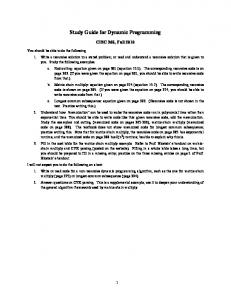
battery’s SOC and the gear position of AMT, and two independent control variables, the engine throttle signal and gear shifting action. The gear is defined as a state in this optimal control problem because it relates directly to the torque of the engine and the shifting action should not be skipped in the control problem. The results of PMP are found to be near-optimal, close to those of DP and the co-state corresponding to the gear position state has an algebraic expression associated with the vehicular speed, which results in the global near-optimal behavior of PMP and gives the major contribution in this paper. The remainder of this paper is organized as follows: in Section 2, the hybrid powertrain is modeled and the optimal control problem is formulated. DP and PMP-based methods are applied and results are analyzed in Section 3. The solutions from DP and PMP are compared in section 4 and the conclusions are provided in Section 5. 2. Hybrid Powertrain Modeling The schematic diagram of the parallel hybrid powertrain and its power flows are shown in Figure 1, where Preq is the power request, Pb is the electric power from the battery pack and Pe is the mechanical power output from the diesel engine, respectively, m f is fuel consumption rate, normally decided by the brake specific fuel consumption (BFSC) map derived through the bench test. The arrows of the lines in Figure 1 indicate the directions of the power flows. The torques of the engine and the electric motor are combined before the AMT. The 7.0 L diesel engine is adopted, giving 155 kW maximum power at the speed of 2000 rpm and 900 Nm maximum output torque within the speed range from 1300 rpm to 1600 rpm. The electric motor can output 90 kW maximum power, 600 Nm maximum torque and has 2400 rpm maximum speed. The 60 Ah lithium-ion battery pack gives 312.5 V rated voltage. The AMT is configured with nine ratios: 12.11, 8.08, 5.93, 4.42, 3.36, 2.41, 1.76, 1.3 and 1. The curb weight of the vehicle is 16,000 kg, the tire radius is 0.508 m, the final ratio is 4.769 and the fronted area is 6.2 m2. Given a driving cycle defined by the vehicle velocity history v (t ) , t ∈[t0,t f ] . The power request Preq (t ) is calculated as in Equation (1): C A 2 P = (δ mv (t ) + fmg cos α (t ) + D v (t ) + mg sin α (t ))v(t ) req 21.15

(1)

where m is the vehicle mass; δ is the mass factor, combining the moving and rotation inertial together; f is the coefficient of the rolling resistance; CD is the aerodynamic coefficient; A is the fronted area; g is the acceleration of the gravity and α (t ) is the gradeability.

At the same time, the power balancing should be maintained, as shown in Equation (2):

Preq (t ) = ( Pe (t ) + Pb (t )ηm )ηT

(2)

where η m is the efficiency of the electric motor, decided by the motor speed and torque, normally derived from the test bench; and η T is the efficiency of the transmission and axle, taken as the constant 0.9. Clearly the engine power Pe (t ) can be regulated by the engine’s throttle signal th(t ) . It means that Pbatt could be decided by th(t ) at any time when Preq (t ) is known in advance. Thus the engine throttle signal th(t ) can be chosen as a control variable, ranging from 0 to 1.

Energies 2013, 6

2308 Figure 1. The pre-transmission parallel hybrid electric powertrain.

m f

Pe

Preq

Pb

The state charge of the battery, soc , relates to the battery current by: 1

so c = −

C b a tt

I (t )

(3)

where Cbatt is the battery capacity; I(t) is the battery current. The variation of soc is calculated by Equation (4): 2

 =− soc

1 Voc ( soc) − Voc ( soc) − 4( Rint ( soc) + Rt ) Pb (t ) Cbatt

2( Rint ( soc) + Rt )

(4)

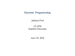
where Voc(soc) is the open circuit voltage; Rint(soc) is the internal resistance of the battery; Rt is the terminal resistance. It should be noted the explicit dependence of soc through open-circuit voltage Voc and the internal resistance Rint. However, the assumption that the variation of soc depends only on Pbatt is made reasonably when soc changes within a narrow range for the hybrid electric vehicles. Voc(soc) and Rint(soc) can be obtain through the bench test, as shown in Figure 2, where soc stays in the primary usage range and thus Voc and Rint can be assumed to be independent of soc.

Energies 2013, 6

2309 Figure 2. Voc and Rint varying as soc changes. 315

0.036 Voc Rint

313

0.033

Primary usage

311

0.03

0.027

307

0.024

305

0.021

303

0.018

V oc

Rint

309

301 0.25

0.3

0.35

0.4

0.45

0.5 soc

0.55

0.6

0.65

0.7

0.015 0.75

The current gear position is defined as a state because the shifting strategy plays a key role for this vehicle and the skip of it is not expected. The variation of current gear position ig (t) , ig (t) ∈{1,2,,9} is associated with gear shifting action sh(t ) and calculated by Equation (5):

ig (t ) = sh(t )

(5)

where sh(t ) can be −1, 0, or 1, representing downshift, hold and upshift, respectively. Over the entire optimization horizon [t0 , t f ] , the system state x(t) = [soc(t), ig (t)]′ evolves according to Equation (6):

x(t) = f (x(t), u(t))

∀t ∈[t0 , t f ]

(6)

where u (t ) = [th(t ), sh(t )]′ , f represents Equations (1–5). The inequality constraints for the state and control variables include: Pb ,min ≤ Pb (t ) ≤ Pb ,max

(7)

ωe ,min ≤ ω e (t ) ≤ ω e ,max

(8)

0 ≤ Pe ( t ) ≤ Pe ,max

(9)

socmin ≤ soc(t ) ≤ socmax

(10)

where Pb,min and Pb,max are the battery recharge and discharge power limitation; ωe ,min (t ) , ωe (t ) and ωe ,max (t ) is the idling speed, normal rotational speed and maximum speed of the engine; Pe,max is the power limitation of the engine; The variable soc(t) is constrained within the permitted minimum value socmin and the maximum value socmax. The cost function to be minimized is normally the compromise of the economy and other performance, here the accumulated fuel consumption and the gear shifting events are included, as shown in Equation (11):

Energies 2013, 6

2310 tf

J =

 [ m

f

( t ) + β sh ( t ) ] d t

(11)

t0

where J is the cost metrics. The portion β sh (t ) is introduced to avoid the excessive shifting and β is a positive weighting factor, here tuned to 0.01 to reach the equilibrium between the shift frequency and fuel consumption [22]. The state terminal conditions are shown in Equation (12):

x(t0 ) = x(t f ) = [0.6, 1]′

(12)

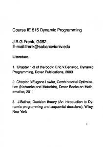
The terminal constraint for x(1) are imposed to ensure battery energy is sustained. The heavy-duty vehicle natural driving cycle used for the simulation is shown in Figure 3, which is obtained from a heavy garbage collecting vehicle under the normal operation full of the frequent stops and brakes. Figure 3. Heavy-duty vehicle natural driving cycle. 70 Heavy Duty Vehicle Cycle 60

Speed (km/h)

50

40

30

20

10

0

0

500

1000

1500

2000

2500

3000

3500

time (sec)

3. Application of DP and PMP

3.1. The DP-Based Numerical Optimization The DP technique solves the multi-step horizon optimization problem based on the Bellman’s principle of optimality and it guarantees the global optimality through exhaustive search of all control and state grids. The principle of optimality dictates that for the discrete system, if u(k ) (k = 0, 1, 2, …, N−1) is the optimal control over the whole problem horizon, then the truncated sequence u(k) (k = s, s+1 ,…, N−1, 0 < s < N) is the optimal control for J ( s ) =

N −1

 {m

k = s +1

J (k ) = min{J (k + 1)) + m f (k ) + β sh(k ) } u(k )

f

( k ) + β sh ( k ) } , which results in:

(13)

When x ( k ) and u(k ) are discretized into the finite states and Equation (13) is solved backwards, the optimal control and corresponding cost are stored and then the optimal solution with the specific initial states is retrieved forwardly by applying the optimal controls through the horizon. However, the

Energies 2013, 6

2311

backward procedure means that the optimal solution can be obtained mostly offline because the driving cycle should be known in advance. The casual control algorithm approximating DP behavior should be pursued in the following practical controller design, which is not covered in the paper. The resolution of soc is 0.01 and the discrete time step is 1 second. The DP algorithm was implemented in MATLAB and applied to obtain the optimal control solution [22].

3.2. The PMP-Based Optimization PMP [23] states that if the control law u * (t ) is optimal for Equation (11), the following conditions should be satisfied as a necessary but not sufficient condition. *

1. The u (t ) minimizes the Hamiltonian H ( x (t ), u (t ), t , p (t )) for all t ∈[t0 , t f ] : *

H ( x (t ), u (t ), t , p (t )) ≥ H ( x (t ), u (t ), t , p (t ))

∀u

(14)

 f (t) + β sh(t) H(x(t), u(t), t, p(t)) = p (t)* f (x(t), u(t)) + m

(15)

where the Hamiltonian is defined as: T

with p (t ) is a vector of the auxiliary variables called co-states and the dimension of p (t ) is the same as x (t ) . 2. The co-state p (t ) satisfies the following equation: p ( t ) = −

∂ H ( x ( t ), u ( t ), t , p ( t )) ∂x

(16)

3. The terminal condition is similar to Equation (12). The conditions given by PMP are only necessary for optimality, but not sufficient. The solution that satisfies the necessary conditions is called the extremal solution. In general, the following two approaches are effective to check whether an extremal solution is sufficient for optimality: (1) The optimal trajectory obtained from PMP is the unique trajectory that satisfies the necessary and boundary conditions; (2) Some geometrical properties of the optimal field provide the possibility of optimality verification, such as the optimal field is convex [21]. In the practical applications, PMP can be used to find the candidate solution through computing and minimizing the Hamiltonian for all t ∈[t0 , t f ] and obtain the extremal controls. The optimal control variables sh(t ) and th (t ) are obtained at each instant to minimize the Hamiltonian, expressed by Equation (17): [ sh * (t ), th * (t )] = arg min H u (t )

(17)

When Equation (6), Equation (15) and Equation (16) are associated, p1 (t ) and p2 (t ) are solved through Equation (18):

Energies 2013, 6

2312 ∂f ( x1 (t )) ∂m f  ( ) ( ) p t = − p t + 1  1 ∂x1 ∂x1    p (t ) = − p (t ) ∂f ( x2 (t )) + ∂m f + β ∂ sh (t ) 2  2 ∂x 2 ∂x 2 ∂x 2

(18)

As the variation of soc depends only on Pb, then the assumption that the co-state p1 (t ) corresponding to soc is a constant can be presented [21], which simplifies the computation tremendously. The co-state p2 (t ) corresponding to the gear shifting is decided by the vehicle velocity and acceleration as in reality. The co-state p (t ) can be solved when Equations (5), (6), (12) and (18) are associated, while enforcing the condition u * (t ) = arg min H to identify a solution candidate. Despite of being completely defined, the two-point boundary values problem can be solved numerically only using an iterative procedure because one boundary condition is defined at the terminal time. The procedure is known as the shooting method and consists of replacing the two-point boundary value problem with a conventional initial-condition problem [24]. An iterative procedure, as shown in Figure 4, has been used to obtain the final values of co-states, making the PMP significantly faster than dynamic programming. It should be noted that similar resolution for soc and the discrete time step as DP are used. The value of co-state p1 (t ) and algebraic expression of p 2 ( t ) associated with vehicle velocity are shown in Equation (19): p1 (t ) ≡ − 3500

0  p 2 (t ) =  − γ γ 

− 1 ≤ v ( k + 1) − v ( k ) ≤ 1 v ( k + 1) − v ( k ) < − 1

(19)

v ( k + 1) − v ( k ) > 1

where γ is determined as 0.011 based on the multiple rounds of the explorations; v(k) is the vehicle speed at k step, when the whole problem is discretized. It should be noted that Equation (19) is dependent on the particular cycles. The value of p1 and γ can be the different value when the cycle changes. The existence and uniqueness of the solutions cannot be proved formally in the general case, but it is reasonable to assume that at least one optimal solution exists for the energy management problem in the sense that there is at least one sequence of controls giving the lowest possible fuel consumption. If the minimum principle generates only one extremal solution, it is the optimal solution. If there is more than one extremal solution, they are all compared and the one yields the lowest total cost is chosen.

Energies 2013, 6

2313 Figure 4. The iterative procedure of PMP.

4. Comparative Analysis for the Results from PMP and DP The SOC curves from DP and PMP respectively are shown in Figure 5. The similar tendency of both curves is found, decreasing first, and then increasing steadily when the engine provides more power. During t = 1500~2000 s, the vehicle operates at the higher velocity, the engine and battery provide the power together and the value of SOC reaches the minimum valley, no matter in DP or PMP case. However, the solutions of DP and PMP have the minor differences. The gear distribution in DP and PMP with the different power requirement and velocity range is shown in Figure 6. Due to the time-varying co-state p2 , which controls the gear shifting in PMP, the result in PMP is basically similar to that in DP. Additionally, the minor difference of the gear shifting is found in Figure 6, as highlighted in the black rectangle area. It can be expressed further in Figure 7. As shown in the green ellipse of Figure 7, the gear in PMP is slightly lower than that in DP, which causes that the operating points of the engine in PMP are mildly lower than those in DP, as noted by the black circles in Figure 8. The total fuel consumption in PMP is slightly more than that in DP can be explained by the operating points of engine and fuel consumption curves in Figure 9. Moreover, the

Energies 2013, 6

2314

difference of the SOC curves in Figure 5 before the minimum valley can be explained by that the power provided by engine in PMP is lower than that in the DP, as shown in Figure 8. Figure 5. SOC curves of DP and PMP. 0.61 DP.SOC PMP.SOC

0.6 0.59

SOC

0.58 0.57 0.56 0.55 0.54 0.53

0

500

1000

1500 2000 time (sec)

2500

3000

3500

Figure 6. Gear distribution of DP and PMP. (a) Gear distribution of DP; (b) Gear distribution of PMP. 150

150 1st gear 2nd gear 3rd gear 4th gear 5th gear 6th gear 7th gear 8th gear 9th gear

100 Power Demand (kW)

Power Demand (kW)

100

50

0

0

10

20

30 40 50 Vehicle Speed (km/h)

(a)

60

70

1st gear 2nd gear 3rd gear 4th gear 5th gear 6th gear 7th gear 8th gear 9th gear

80

50

0

0

10

20

30 40 50 Vehicle Speed (km/h)

(b)

60

70

80

Energies 2013, 6

2315 Figure 7. Gear shifting of DP and PMP.

10 gear of DP gear difference between DP and PMP

9

8

7

6

gear

5

4

3

2

1

0

-1

0

500

1000

1500

2000

2500

3000

3500

time (sec)

Figure 8. Work area of engine in DP and PMP. (a) Working zone of the engine in DP; (b) Working zone of the engine in PMP. 21

900

0

0

21

900

20

500

20 0

205 21 0

300 220

220 230

230

200 100

1000

22 0 230

24 0 25 0 240 26 0 250 270 280 260 270 0 30 280 31 0 3300 3000 34 31 00 35 36 00 3738 00 33 34 00 35 39 4000 36 37380 0 42 5 1200 1400 1600 1800 Ening Speed /rpm

(a)

2000

24 0 25 0 26 0 27 0 280 300 310 330 340 000 35 36 3738 0 394000 42 5 45 0 5 47 0 50 2200

20

500

20 0

20 5 21 0

21 0

205 21 0

300 220

220 230

230

200 100 0 800

0

0

20 5

400

0

0

20 5 21 0

21 0

0 800

20

600 0

20 5

400

700

E ngine T orque /Nm

E ngine T orque /Nm

600

0

21

20

800

21

700

20 5

20 5

800

1000

22 0 230

24 0 25 0 240 26 0 250 270 280 260 270 0 30 280 31 0 3000 3300 34 31 00 35 36 00 3738 00 33 34 0 39 35 4000 00 36 3738 42 5 0 1200 1400 1600 1800 Ening Speed /rpm

2000

24 0 25 0 26 0 27 0 280 300 310 330 340 000 35 36 3738 0 394000 42 5 45 0 5 47 0 50 2200

(b)

Consequently, it is significant to observe that when tuned with an appropriate co-state value, PMP can give a solution close to DP although it has been implemented with an instantaneous minimization

Energies 2013, 6

2316

process. The co-states p1 and p2 are compared with the analogue quantities extracted from DP in Figures 9 and 10 respectively, according to Equation (20) [23]:

J x* ( x* (t ), t ) = p* (t )

(20)

where J x∗ ( x∗ (t ), t ) is the partial derivative of the cost function J with the respect to x when the optimal trajectory x*(t) is adopted, p*(t) is the optimal co-state trajectory. It is found that co-states generated by the iterative procedure as shown in Figure 4 and Equation (19) approximate the optimal solution from DP effectively. It also explains the similar behavior of DP and PMP as shown in Figures 6–8. The fuel consumption in the PMP case is 5.37L, 0.4% more than that of 5.35L in DP case. Figure 9. J ∗ x1 and p1. 1

Relative error /%

-3505

J*x and p 1

-3495

1

0 -3500

J*

x

1

p

1

Relative error -3505 0

500

1000

1500

t /sec

2000

2500

-1 3500

3000

Figure 10. J ∗x2 and p2. 0.015

7

0.01

Absolute error /10-4

0 -0.005

2

J*x and p 2

0.005

-0.01 -0.015

J*

-0.02

p

x

2

-0.025 0

2

Absolute error 500

1000

1500

t /sec

2000

2500

3000

-3 3500

5. Conclusions The DP and PMP techniques are used to obtain the energy management algorithm for a parallel HEV with AMT. The PMP was demonstrated to be effective in generating near-optimal results, close to those of DP, even though it has been implemented with an instantaneous minimization process. The constant co-state assumption associated with SOC doesn’t influence the gear position state in the

Energies 2013, 6

2317

results considerably. The co-state p2 (t ) corresponding to the gear position state ig (t) has an algebraic expression associated with the velocity, which results in the global optimal behavior of PMP and is the major contribution in this paper. Additionally, the total fuel consumption in the PMP case is close to that in DP. On the other hand, PMP can save the approximately 77% time of DP, including the iteration to approximate the co-states. Future research efforts will find another quadratic function of the co-state p2 (t ) associated with the velocity and acceleration, and estimating the co-state p2 (t ) online to adapt the gear position state to the driver’s style and actual drive cycle. Acknowledgements This work is supported by the Natural Science Foundation of China (Grant No. 50905015) and University Discipline Talent Introduction Program (Grant No. B12022). The authors express their gratitude for the valuable suggestions and advice from the anonymous reviewers. References Sciarretta, A.; Guzzella, L. Control of hybrid electric vehicles. IEEE Control Syst. Mag. 2007, 27, 60–70. 2. Serrao, L.; Onori, S.; Rizzoni, G.; Guezennec, Y. A Novel Model-Based Algorithm for Battery Prognosis. In Proceedings of the Seventh IFAC Symposium on Fault Detection, Supervision and Safety of Technical Processes, Barcelona, Spain, 30 June–3 July 2009. 3. Brahma, A.; Guezennec, Y.; Rizzoni, G. Optimal Energy Management in Series Hybrid Electric Vehicles. In Proceedings of the 2000 American Control Conference, Columbus, OH, USA, 28–30 June 2000; pp. 60–64. 4. Lin, C.-C.; Peng, H.; Grizzle, J.W.; Kang, J.-M. Power management strategy for a parallel hybrid electric truck. IEEE Trans. Control Syst. Technol. 2003, 11, 839–849. 5. Sundström, O.; Ambühl, D.; Guzzella, L. On implementation of dynamic programming for optimal control problems with final state constraints. Oil Gas Sci. Technol. 2009, 65, 91–102. 6. Anatone, M.; Cipollone, R.; Sciarretta, A. Control-Oriented Modeling and Fuel Optimal Control of a Series Hybrid Bus; SAE Technical Paper 2005-01-1163; SAE International: Warrendale, PA, USA, 2005; doi:10.4271/2005-01-1163. 7. Wei, X.; Guzzella, L.; Utkin, V.; Rizzoni, G. Model-based fuel optimal control of hybrid electric vehicle using variable structure control systems. J. Dyn. Syst. Meas. Control 2007, 129, 13–19. 8. Serrao, L.; Rizzoni, G. Optimal Control of Power Split for a Hybrid Electric Refuse Vehicle. In Proceedings of the 2008 American Control Conference, Seattle, WA, USA, 11–13 June 2008; pp. 4498–4503. 9. Johannesson, L.; Åsbogård, M.; Egardt, B. Assessing the potential of predictive control for hybrid vehicle powertrains using stochastic dynamic programming. IEEE Trans. Intell. Transp. Syst. 2007, 8, 71–83. 10. Tate, E.; Grizzle, J.; Peng, H. Shortest path stochastic control for hybrid electric vehicles. Int. J. Robust Nonlinear Control 2008, 18, 1409–1429. 1.

Energies 2013, 6

2318

11. Borhan, H.; Vahidi, A.; Phillips, A.; Kuang, M.; Kolmanovsky, I. Predictive Energy Management of a Power-Split Hybrid Electric Vehicle. In Proceedings of the 2009 American Control Conference, St. Louis, MO, USA, 10–12 June 2009. 12. Jeon, S.I.; Jo, S.T.; Park, Y.I.; Lee, J.M. Multi-mode driving control of a parallel hybrid electric vehicle using driving pattern recognition. J. Dyn. Syst. Meas. Control 2002, 124, 141–149. 13. Delprat, S.; Guerra, T.M.; Rmaux, J. Control Strategies for Hybrid Vehicles: Optimal Control. In Proceedings of Vehicular Technology Conference, 2002 (VTC 2002-Fall). Vancouver, Canada, 24–28 September 2002; pp. 1681–1685. 14. Delprat, S.; Lauber, J.; Marie, T.; Rimaux, J. Control of a paralleled hybrid powertrain: Optimal control. IEEE Trans. Veh. Technol. 2004, 53, 872–881. 15. Rousseau, G.; Sinoquet, D.; Rouchon, P. Constrained optimization of energy management for a mild-hybrid vehicle. Oil-Gas Sci. Technol. IFP 2007, 62, 623–624. 16. Cipollone, R.; Sciarretta, A. Analysis of the Potential Performance of a Combined Hybrid Vehicle with Optimal Supervisory Control. In Proceedings of the 2006 IEEE International Conference on Control Applications, Munich, Germany, 4–6 October; pp.2802–2807. 17. Sciarretta, A.; Back, M.; Guzzella, L. Optimal control of paralleled hybrid electric vehicles. IEEE Trans. Control Syst. Technol. 2004, 12, 352–363. 18. Guzzella, L.; Sciarretta, A. Vehicle Propulsion Systems: Introduction to Modeling and Optimization; Springer-Verlag: Berlin, Germany, 2005; pp. 208–225. 19. Musardo, C.; Rizzoni, G.; Guezennec, Y.; Staccia, B. A-ECMS: An adaptive algorithm for hybrid electric vehicle energy management. Eur. J. Control 2005, 11, 509–524. 20. Serrao, L.; Onori, S.; Rizzoni, G. A comparative analysis of energy management strategies for hybrid electric vehicles. J. Dyn. Syst. Meas. Control 2011, 133, 031012:1–031012:9. 21. Kim, N.; Cha, S.; Peng, H. Optimal control of hybrid electric vehicles based on Pontryagin’s minimum principle. IEEE Trans. Control Syst. Technol. 2011, 19, 1279–1287. 22. Zou, Y.; Hou, S.J.; Li, D.G.; Gao, W.; Hu, X.S. Optimal energy control strategy design for a hybrid electric vehicle. Discret. Dyn. Nat. Soc. 2013, doi:10.1155/2013/132064. 23. Kirk, D.E. Optimal Control Theory: An Introduction; Dover Publications Incorporated: Mineola, NY, USA, 2004; pp. 227–240. 24. Krotov, V.F. Global Methods in Optimal Control Theory; Marcel Dekker, Inc: New York, NY, USA, 1996; p. 140. © 2013 by the authors; licensee MDPI, Basel, Switzerland. This article is an open access article distributed under the terms and conditions of the Creative Commons Attribution license (http://creativecommons.org/licenses/by/3.0/).