Nov 12, 2010 - thesis research, with a focus on gear-shaft-bearing structural analysis, ..... Figure3.15 Effect of pilot bearing position on line-of-action vector for ...
UNIVERSITY OF CINCINNATI Date: 2-Nov-2010 I, Xia Hua
,
hereby submit this original work as part of the requirements for the degree of:
Master of Science in
Mechanical Engineering
It is entitled:
Hypoid and Spiral Bevel Gear Dynamics with Emphasis on Gear-Shaft-Bearing Structural Analysis
Student Signature:
Xia Hua
This work and its defense approved by: Committee Chair:
11/12/2010
Teik Lim, PhD Teik Lim, PhD
1,173
Hypoid and Spiral Bevel Gear Dynamics with Emphasis on Gear-Shaft-Bearing Structural Analysis
A thesis submitted to the Division of Research and Advanced Studies of the University of Cincinnati in partial fulfillment of the requirements for the degree of MASTER OF SCIENCE in the Program of Mechanical Engineering of the College of Engineering and Applied Science
November 2010 by Xia Hua
B.S. Zhejiang University of Technology, Zhejiang, P.R. China, 2007
Academic Committee Chair: Members:
Dr. Teik C. Lim Dr. Ronald Huston Dr. David Thompson
ABSTRACT Hypoid and spiral bevel gears, used in the rear axles of cars, trucks and offhighway equipment, are subjected to harmful dynamic response which can be substantially affected by the structural characteristics of the shafts and bearings. This thesis research, with a focus on gear-shaft-bearing structural analysis, is aimed to develop effective mathematical models and advanced analytical approaches to achieve more accurate prediction of gear dynamic response as well as to investigate the underlying physics affecting dynamic response generation and transmissibility. Two key parts in my thesis are discussed below. Firstly, existing lumped parameter dynamic model has been shown to be an effective tool for dynamic analysis of spiral bevel geared rotor system. This model is appropriate for fast computation and convenient analysis, but due to the limited degrees of freedom used, it may not fully take into consideration the shaft-bearing structural dynamic characteristics. Thus, a dynamic finite element model is proposed to fully account for the shaft-bearing dynamic characteristics. In addition, the existing equivalent lumped parameter synthesis approach used in the lumped parameter model, which is key to representing the shaft-bearing structural dynamic characteristics, has not been completely validated yet. The proposed finite element model is used to guide the validation and improvement of the current lumped parameter synthesis method using effective mass and inertia formulations, especially for modal response that is coupled to the pinion or gear bending response. Secondly, a new shaft-bearing model has been proposed for the effective supporting stiffness calculation applied in the lumped parameter dynamic analysis of the
iii
spiral bevel geared rotor system with 3-bearing straddle-mounted pinion configuration. Also, based on 14 degrees of freedom lumped parameter dynamic model and quasi-static three-dimensional finite element tooth contact analysis program, two typical shaftbearing configuration used in automotive application, that are the 3-bearing straddle mounted pinion configuration and the 2-bearing overhung mounted pinion configuration, are compared for their different contribution to the spiral bevel gear mesh and dynamics. Parametric study is also performed to analyze the effect of shaft-bearing configuration on spiral bevel gear mesh and dynamics.
iv
v
ACKNOWLEGEMENTS First of all, I would like to sincerely thank my advisor and committee chair, Dr. Teik C. Lim, for his guidance and support during my graduate study thus far. Also, my gratitude is expressed to Dr. David Thompson and Dr. Ronald Huston for serving as my master supervisory committee members. This thesis research is supported by the Hypoid and Bevel Gear Mesh and Dynamic Modeling Consortium. In addition, I wish to thank all my labmates at the Vibro-Acoustic and Sound Quality Research Laboratory, University of Cincinnati for their cooperation and help. Finally, I should thank my parents and my wife Gaoyan Shi for their love and encouragement during my study.
vi
CONTENTS Chapter 1. Introduction ....................................................................................................... 1 1.1 Literature Review...................................................................................................... 2 1.2 Motivation, Objectives and Thesis Organization...................................................... 4 Chapter 2. Finite Element and Enhanced Lumped Parameter Dynamic Modeling of Spiral Bevel Geared Rotor System ..................................................................................... 6 2.1 Introduction ............................................................................................................... 6 2.2 Proposed Dynamic Finite Element Model ................................................................ 7 2.3 Proposed New Lumped Parameter Synthesis Method for Existing Lumped Parameter Dynamic Model and Its Difference from the Old Lumped Parameter Synthesis Approach ...................................................................................................... 13 2.3.1 Spiral Bevel Gear 14-DOF Lumped Parameter Dynamic Model .................... 13 2.3.2 Proposed New Lumped Parameter Synthesis Method in Spiral Bevel Gear ... 16 14 DOF Lumped Parameter Model........................................................................... 16 2.3.3 Difference Between Old Lumped Parameter Synthesis Approach and Proposed New Lumped Parameter Synthesis Approach .......................................................... 28 2.4 Comparison Results and Discussions ..................................................................... 28 2.5 Conclusion .............................................................................................................. 35 Chapter 3. Effect of Shaft-bearing Configurations on Spiral Bevel Gear Mesh and Dynamics .......................................................................................................................... 36 3.1 Introduction ............................................................................................................. 36 3.2 Mathematical Model ............................................................................................... 37 3.2.1 Mesh Model ..................................................................................................... 37 3.2.2 Spiral Bevel Gear 14-DOF Lumped Parameter Dynamic Model .................... 38 3.2.3 Finite Element Modeling of 3-bearing Straddle Mounted Pinion Configuration for the Effective Lumped Stiffness Calculation........................................................ 41 3.2.4 Axial Translational Stiffness Model Refinement ............................................ 44 3.3 Comparison of 3-bearing Straddle Mounted Pinion and 2-bearing Overhung Mounted Pinion on Gear Mesh and Dynamics ............................................................. 46 3.3.1 Analysis on Equivalent Shaft-bearing Stiffness Models and Pinion‘s Lumped Shaft-bearing Stiffness Matrices of Two Pinion Configurations .............................. 49 3.3.2 Comparison on Gear Dynamics ....................................................................... 52 3.3.3 Effect of 2-bearing and 3-bearing Configurations on Mesh Model ................. 57 3.4 Conclusions ............................................................................................................ 70 Chapter 4. Conclusions ..................................................................................................... 72 BIBLIOGRAPHY ............................................................................................................. 74
vii
LIST OF FIGURES Figure2.1 Dynamic finite element model of spiral bevel geared rotor system ................... 8 Figure2.2 Spiral bevel gear pair dynamic model ............................................................. 11 Figure2.3 Spiral bevel gear 14 DOF lumped parameter dynamic model ....................... 16 Figure2.4 Static finite element modeling of 3-bearing straddle mounted pinion configuration ..................................................................................................................... 19 Figure2.5 Axial translational stiffness model ................................................................... 20 Figure2.6 A design of beam with lumped mass ................................................................ 21 Figure2.7 Beam with lumped mass model of pinion with integrated shaft....................... 23 Figure2.8 Dynamic mesh forces ....................................................................................... 30 Figure2.9 Dynamic mesh forces ....................................................................................... 31 Figure2.10 Dynamic mesh forces ..................................................................................... 32 Figure2.11 Dynamic mesh forces ..................................................................................... 34 Figure2.12 Dynamic mesh forces ..................................................................................... 34 Figure2.13 Dynamic mesh forces ..................................................................................... 35 Figure3.1 Tooth load distribution generated from quasi-static three-dimensional finite element tooth contact analysis program ........................................................................... 38 Figure3.2 Spiral bevel gear 14 DOF lumped parameter dynamic model ........................ 41 Figure3.3 Static finite element modeling of 3-bearing straddle mounted pinion configuration ..................................................................................................................... 44 Figure3.4 Axial translational stiffness model ................................................................... 45 Figure3.5 3-bearing straddle mounted pinion (upper) and 2-bearing overhung mounted pinion (lower).................................................................................................................... 49 Figure3.6 Finite element model of 3-bearing mounted pinion (left) and finite element model of 2-bearing mounted pinion (right) ...................................................................... 52 Figure3.7 Comparison of 2-bearing and 3-bearing configurations on dynamic mesh force .................................................................................................................................. 53 Figure3.8 Comparison of 2-bearing and 3-bearing configurations on modal strain energy distribution ........................................................................................................................ 54 Figure3.9 Comparison of 2-bearing and 3-bearing configurations on dynamic bearing load ................................................................................................................................... 56 Figure3.10 Comparison of 2-bearing and 3-bearing configurations on pinion response 57 Figure3.11 Effect of pilot bearing position on mesh point for 3-bearing case................. 58 Figure3.12 Effect of tapered roller bearing position on mesh point for 3-bearing case.. 59 Figure3.13 Effect of tapered roller bearing position on mesh point for 2-bearing case.. 60 Figure3.14 Comparison of 2-bearing and 3-bearing configurations on mesh point ....... 61 Figure3.15 Effect of pilot bearing position on line-of-action vector for 3-bearing case . 62 Figure3.16 Effect of tapered roller bearing position on line-of-action vector for 3bearing case ...................................................................................................................... 63 Figure3.17 Effect of tapered roller bearing position on line-of-action vector for 2bearing case ...................................................................................................................... 64 Figure3.18 Comparison of 2-bearing and 3-bearing configuration on line-of-action vector................................................................................................................................. 65 Figure3.19 Effect of pilot bearing position on mesh stiffness for 3-bearing case ............ 66
viii
Figure3.20 Effect of tapered roller bearing position on mesh stiffness for 3-bearing case ........................................................................................................................................... 67 Figure3.21 Effect of tapered roller bearing position on mesh stiffness for 2-bearing case ........................................................................................................................................... 67 Figure3.22 Comparison of 2-bearing and 3-bearing configuration on mesh stiffness .... 68 Figure3.23 Comparison on dynamic mesh force without considering the difference of mesh stiffness .................................................................................................................... 69 Figure3.24 Comparison on dynamic mesh force considering the difference of mesh stiffness.............................................................................................................................. 69
ix
Chapter 1. Introduction Hypoid and spiral bevel gears are widely used as final set of reduction gear pairs in the rear axles of trucks, cars and off-highway equipment to transmit engine‘s power to the drive wheels in non-parallel directions. The hypoid and spiral bevel gear dynamics becomes more and more significant for the concern of noise and durability, because under dynamic condition the mesh force acting on gear teeth are amplified which potentially reduces the fatigue life of gears and the large dynamic force can be transmitted to housing which causes structure-born gear whine. Accordingly, it is needed to perform in-depth investigation on hypoid and spiral bevel geared system dynamic response and resonance characteristics to form a deeper understanding in the physics controlling dynamic force generation and transmissibility to achieve superior design for quiet and durable driveline. Though it is the fact that much is known about dynamic characteristics in parallel axis gear system, research on the dynamics of nonparallel axis geared systems such as hypoid and spiral bevel gears is not mature. Most previous analytical work mainly focuses on gear mesh modeling and its application to analyze gear pair dynamics, nonlinear time-varying gear pair dynamic analysis considering gear backlash, time-varying mesh characteristics, mesh stiffness asymmetry effects and friction, coupled multi-body gear pair dynamic and vibration analysis and so on. Very little amount of attention is given to the gear-shaft-bearing structure of the geared rotor system. The goal of this thesis is to gain a better understanding on the effect of gear-shaft-bearing structural design on hypoid and spiral bevel gear system dynamics and to establish new computational models more accurately accounting for gear-shaft-bearing dynamic characteristics.
1
1.1 Literature Review Dynamics of parallel axis geared rotor system has been studied extensively[1-14]. Papers by Ozguven and Houser[1] and Blankenship and Singh[2] provide a comprehensive review of mathematical models used to investigate dynamics of parallel axis geared rotor system. Among these studies, a special attention has been paid on gearshaft-bearing structure rather than the dynamics of the gear itself. In 1975, Mitchell and Mellen[3] indicate the torsional-lateral coupling in a geared rotor system by conducting experiment study. In 1981, Hagiwara, Ida[4] analytically and experimentally studied the vibration of geared shafts due to run-out unbalanced and run-out errors and it is observed that both torsional and lateral modes could be excited by gear errors and unbalanced forces. In 1984, Neriya, Bhat and Sankar[5] studied the effect of coupled torsionalflexural vibration of a geared shaft system on dynamic tooth load by using lumped parameter dynamic model in which equivalent lumped springs were used to represent the flexibility of shaft-bearing structure. In 1985, Neriya, Bhat and Sankar[6] used finite element method to model the geared rotor system and introduced the coupling between torsion and flexure at the gear pair location. In 1991, Lim and Singh[7] developed linear time-invariant, discrete dynamic models of a generic geared rotor system based on their newly proposed bearing matrix formulation by using lumped parameter and dynamic finite element techniques to predict the vibration transmissibility through bearing and mounts, casing vibration motion, and dynamic response of the internal rotating system. In 2004, Kubur and Kahraman[8] proposed a dynamic model of a multi-shaft helical gear reduction unit formed by N flexible shafts by finite elements. This model has an accurate
2
representation of shafts and bearings as well as gears, which is used to study the influence of some key gear-shaft-bearing structure parameters. Though large numbers of research has been done on parallel axis gear dynamics, the research on dynamics of right-angle geared rotor system such as bevel and hypoid gear is still scanty. In recent years, a group led by Lim[15-19] began to develop the dynamic model of right-angle hypoid and spiral bevel geared rotor system and analyze the dynamic characteristics of hypoid and spiral bevel geared rotor system. In one of the study, Cheng and Lim[15] developed the single-point gear mesh-coupling model based on both unloaded and loaded exact gear tooth contact analysis. This mesh model is then applied to develop multiple degrees-of-freedom, lumped parameter model of the hypoid and spiral bevel geared rotor system for linear time-invariant and nonlinear time-varying analysis. In 2002, Wang, H. and Lim[16] developed a multi-point gear mesh-coupling model based on Cheng‘ single point gear mesh-coupling model and applied it to dynamic analysis of hypoid and spiral bevel geared rotor system. In the same year, Jiang and Lim[17] formulated a low degrees of freedom torsional dynamic model to analyze the nonlinear phenomenon through both analytical and numerical solutions. In 2007, based on the low degrees of freedom torsional dynamic model, Wang, J. and Lim[18] extended Jiang‘s work and further investigated the influence of time-varying mesh parameters and various nonlinearities on gear dynamics. In 2010, through developing various more accurate high degrees of freedom lumped parameter dynamic models, Tao and Lim[19] examines torque load effect on gear mesh and nonlinear time-varying dynamic responses, coupled multi-body dynamics and vibration, influence of the typical rotor dynamic factor
3
on hypoid gear vibration, effect of manufacturing error or assembly error on gear dynamics and the interaction between internal and external excitations.
1.2 Motivation, Objectives and Thesis Organization From above literature review, it could be observed that most of the research on hypoid and bevel geared rotor system dynamics is concerned with gear mesh dynamics so the flexibility of gear-shaft-bearing structure is simply represented by equivalent supporting springs or even ignored in much study only focusing on the effect of gear mesh characteristics. Very little attention has been paid to the detailed modeling and analysis of gear-shaft-bearing structure for the concern of dynamics of the whole geared rotor system. Therefore, in this thesis, an attention will be given to the gear-shaft-bearing structural analysis to achieve more accurate prediction of gear dynamic response and to investigate the effect of shaft and bearing design on gear dynamics. Chapter 1 presents the general introduction, literature review, motivation and objective for this thesis research. It discusses current progress in gear dynamics research and the limitations of the research on hypoid and spiral bevel gear dynamics. The discussion further illustrates the objectives of this thesis, which is to perform study on dynamics of hypoid and spiral bevel geared rotor system with emphasis on the gear-shaftbearing structural modeling and analysis. Chapter 2 proposes a finite element dynamic model of hypoid and spiral bevel geared rotor system to fully account for dynamic characteristics of gear-shaft-bearing structure. In addition, the proposed finite element dynamic model is used to guide the improvement of the existing lumped parameter dynamic model using effective mass and
4
inertia formulations, especially for modal response that are coupled to the pinion or gear bending. Chapter 3 proposes a new shaft-bearing model for the effective supporting stiffness calculation for the lumped parameter dynamic analysis of the hypoid and spiral bevel geared rotor system with 3-bearing straddle-mounted pinion configuration. In addition, two typical gear-shaft-bearing configurations used in automotive application are compared for their different contribution to the hypoid and spiral bevel gear mesh and dynamics. Parametric study is also performed to analyze the effect of gear-shaft-bearing configuration on gear mesh and dynamics. Chapter 4 gives a summary of the significant achievement of this thesis research and the recommendations for future work.
5
Chapter 2. Finite Element and Enhanced Lumped Parameter Dynamic Modeling of Spiral Bevel Geared Rotor System
2.1 Introduction Along with the operating speed of geared rotor system growing higher, the dynamics of geared system becomes more and more significant for the concern of noise and durability, because under dynamic condition the mesh force acting on gear teeth are amplified which potentially reduces the fatigue life of gears and the large dynamic force can be transmitted to housing which causes structure-born gear whine. Dynamics of gear systems have been studied extensively [1-14]. Though it is the fact that much is known about dynamic characteristics in parallel axis gear system, research on the dynamics of nonparallel axis geared systems such as hypoid and spiral bevel gears is not mature. In recent years, a group led by Lim [15-19] began to develop the dynamic model of spiral bevel geared rotor system and analyze the dynamic characteristics of spiral bevel geared rotor system. In one of the study, Cheng and Lim [15] developed the single-point gear mesh-coupling model based on the exact spiral bevel gear geometry. This mesh model is then applied to develop multiple degrees-of-freedom, lumped parameter model of the spiral bevel geared rotor system. Later, based on this model, Tao and Lim [19] investigated the influence of various gear system parameters on dynamic characteristics of the spiral bevel geared rotor system. However, due to limited degrees of freedom, the lumped parameter model may not fully take into account the shaft-bearing dynamic characteristics and also the lumped parameter synthesis method used in this model is not mature.
6
In this paper, two modeling methods of spiral bevel geared rotor dynamic system, i.e. the finite element dynamic modeling and the enhanced equivalent lumped parameter synthesis, are introduced and compared. This first objective of this paper is to develop a dynamic finite element model which could better take into account and describe the shaft-bearing dynamic characteristics than the multiple degrees-of-freedom, lumped parameter dynamic model [15]. The second objective is to develop a more accurate lumped point parameter synthesis method fully considering the shaft-bearing structural characteristics in existing lumped parameter model [15] and compare with the proposed dynamic finite element model.
2.2 Proposed Dynamic Finite Element Model As shown in Figure2.1, the mass/inertia of the pinion head and ring gear is separately lumped at one node and the two nodes have mesh coupling between them. The mass/inertia of the differential is lumped at one node. The pinion shaft and gear shaft are modeled with beam elements, for which consistent mass matrix is used. The bearings are modeled as stiffness matrices according to a bearing stiffness formulation[21,22]. The engine and load are separately represented by one node. All nodes of the system respectively have 6 DOFs except for the two nodes representing the engine and load which only have torsional DOFs. The system totally has 17 nodes and accordingly 6 *15 1* 2 92 DOFs.
7
Figure2.1 Dynamic finite element model of spiral bevel geared rotor system The stiffness and mass matrices of each beam element are determined and assembled to form stiffness [ K sp ] and mass [ M sp ] matrices of pinion shaft and stiffness [ K sg ] and mass [ M sg ] matrices of gear shaft. Overall shaft stiffness and mass matrices
of
the
system
are
then
assembled
as
[ K s ] Diag[[ K sp ][ K sg ]]
and
[M s ] Diag[[M sp ][M sg ]].
The engine and load are separately connected to one node at pinion shaft and one node at gear shaft with torsional springs. The stiffness matrices of the torsional spring elements used to connect the engine and pinion shaft and to connect the load and gear
8
shaft could be written in terms of individual torsional spring stiffness as [ K tsp ] and [ K tsg ] , both of which are 7 by 7. The overall stiffness matrices of torsional spring elements of the whole system could be written as [ K ts ] Diag[[ K tsp ][ K tsg ]]. The overall mass matrices of engine and load of the whole system could be written in terms of torsional moment of inertia of engine and load I E , I L as [M E , L ] Diag[ I E I L ]. In industry, pinion shaft is usually supported by 2 or 3 bearings and gear shaft is usually supported by 2 bearings. Suppose that the system has a total of n bearings, the overall bearing stiffness matrix of the whole system could be written by assembling the individual
bearing
element
stiffness
matrices
[ K bi ](i 1 to n)
as
[ K b ] [[ K b1 ][ K b 2 ][ K b3 ][ K bn ]].
The gear stiffness coupling matrix which represents the mesh coupling between the two nodes representing pinion head and ring gear could be derived from the free vibration equations of motion of spiral bevel gear pair. The dynamic model of the spiral bevel gear pair is shown in Figure2.2. The pinion and gear, which are both built as rigid body, are connected by linear gear mesh spring and damper. Using a quasi-static threedimensional finite element tooth contact analysis program[23,24] and concept of contact cells[15], the averaged mesh point, averaged line-of-action, averaged mesh stiffness and loaded transmission error are obtained to represent the mesh spring connecting point, mesh spring direction , mesh spring stiffness and transmission error excitation between pinion and gear. Pinion and gear are both allowed to move in 6 directions so the gear pair dynamic system totally has 12 degrees of freedom. The generalized coordinates of pinion and
gear
are
separately
9
expressed
as
{q pg } {x p , y p , z p , px , py , pz , x g , y g , z g , gx , gy , gz }T . The undamped free vibration
equations of motion for this gear pair dynamic system could be expressed as: m p xp k m pn px 0 m p y p k m pn py 0 m p zp k m pn pz 0 I pxpx k m pn pz y pm k m pn py z pm 0 I pypy k m pn px z pm k m pn pz x pm 0 I pzpz k m pn py x pm k m pn px y pm 0 m g xg k m pn gx 0
(1)
m g yg k m pn gy 0 m g zg k m pn gz 0 I gxgx k m pn gz y gm k m pn gy z gm 0 I gygy k m pn gx z gm k m pn gz x gm 0 I gzgz k m pn gy x gm k m pn gx y gm 0
where, (nlx , nly , nlz ) is the line-of-action vector, ( xlm , ylm , z lm ) (l p, q) is the mesh point vector. l p, q refers to pinion and gear local coordinate systems respectively. k m is mesh stiffness. p is relative displacement between pinion and gear along line-of-action and is expressed as: p x g n gx y g n gy z g n gz gx y gm n gz gx z gm n gy gy z gm n gx gy x gm n gz gz x gm n gy gz y gm n gx x p n px y p n py z p n pz px y pm n pz px z pm n py
(2)
py z pm n px py x pm n pz pz x pm n py pz y pm n px
Combining equations (1-2), a clearer equation of motion could be obtained as: [m pg ]{qpg } [k pg ]{q pg } 0
(3)
here, [m pg ] diag[m p , m p , m p , I px , I py , I pz , mg , mg , mg , I gx , I gy , I gz ]
10
(4)
k m {h p }T {h p } k m {h p }T {hg } [k pg ] k m {hg }T {h p } k m {hg }T {hg }
(5)
Here, {h p } and {hg } are the coordinate transformation vectors between the spiral bevel gear line-of-action direction and generalized coordinate directions for pinion and gear separately. They are expressed as: {hl } {nlx , nly , nlz , lx , ly , lz }(l p, q) ,
(6)
{lx , ly , lz } { yl nlz - zl nly , zl nlx xl nlz , xl nly yl nlx }(l p, q) .
(7)
Figure2.2 Spiral bevel gear pair dynamic model The gear mesh stiffness matrix [k pg ] and the mass matrix [m pg ] of the gear pair can be obtained from Equations (3-7). The overall gear mesh stiffness and mass matrices of
the
whole
system
could
be
obtained
[M pg ] Diag[[m pg ]] .
11
as
[ K pg ] Diag[[k pg ]]
and
The mass and stiffness matrices of the whole dynamic finite element system are derived as [M ] [M pg ] [M s ] [M E ,L ] , [ K ] [ K pg ] [ K s ] [ K b ] [ K ts ]. The system proportional damping is assumed in this model as [C ] s ([ K s ] [ K b ] [ K ts ]) m [ K pg ]
(8)
where, s is the system damping ratio, m is the mesh damping ratio. The excitation of the whole system could be written as {F (t )} [{h p } {hg }]T (k m cm j )e(t )
(9)
The equation of motion of the whole spiral bevel geared rotor system could be expressed as [M ]{X (t )} [C ]{X (t )} [ K ]{X (t )} {F (t )} .
(10)
The direct method is applied here to calculate the steady state forced response as {X (t )} [ H ( )]1{F (t )} .
(11)
The dynamic response of pinion head and ring gear could be derived from X (t ) as
X
p
},{ X g }. The dynamic transmission error is expressed as
d {h p }{X p} {hg }{X g }.
(12)
The dynamic mesh force in line-of-action direction is expressed as
Fm k m ( d 0 ) cm (d 0 ) .
(13)
where, k m is mesh stiffness; cm m k m is mesh damping; 0 is loaded transmission error. The given spiral bevel geared rotor system in Figure2.1 is an example used to explain proposed dynamic finite element modeling theory. The same theory could be
12
applied to spiral bevel geared rotor system with other kinds of pinion or gear configurations.
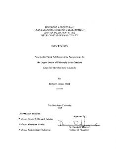
2.3 Proposed New Lumped Parameter Synthesis Method for Existing Lumped Parameter Dynamic Model and Its Difference from the Old Lumped Parameter Synthesis Approach 2.3.1 Spiral Bevel Gear 14-DOF Lumped Parameter Dynamic Model The spiral bevel gear 14-DOF lumped parameter dynamic model[15] used in this study comprises of a spiral bevel gear pair, an engine element and a load element as shown in Figure2.3. Engine and load respectively have 1 DOF which is torsional coordinate. Pinion and gear are both modeled as rigid body which separately have 6 DOFs. Torsional springs are used to connect pinion and engine as well as to attach gear and load. Pinion and gear have mesh coupling. k m is the averaged mesh stiffness and TE is the static transmission error. Since pinion and gear are built as rigid body, their mass and inertia are lumped at each lumped point. Lumped shaft-bearing springs are connected to each lumped point of pinion and gear to support pinion and gear. The equation of motion could be expressed as: [M ]{q} [C]{q} [ K ]{q} {F (t )}
(14)
The generalized coordinates are expressed as: {q} { E ,{q p }T ,{q g }T , L }T
(15)
{ql } {xl , yl , zl . ,lx ,ly ,lz }T (l = p, g) . The lumped mass matrix is described as: 13
(16)
[ M ] diag [ I E , M px , M py , M pz , I px , I py , I pz , M gx , M gy , M gz , I gx , I gy , I gz , I L ] [ K ] Diag[[ K ll ]] Diag[[ K pg ]] Diag[[ K tsp ][ K tsg ]]
(17)
(18)
Here, [ K ll ] is the lumped shaft-bearing stiffness matrix of pinion and gear. [ K pg ] is the gear mesh coupling stiffness matrix. [ K tsp ] is the coupling stiffness
matrix of the torsional spring used to connect pinion and engine. [ K tsg ] is the coupling stiffness matrix of the torsional spring used to connect gear and load. The damping [C] is assumed to be system proportional, which is expressed as: [C ] s ( Diag[[ K ll ]] Diag[[ K tsp ][ K tsg ]]) m Diag[[ K pg ]] (19)
where s is system damping ratio and m is mesh damping ratio. The force vector {F (t )} at the right side of Equation (14) is, {F (t )} [{h p },{hg }]T (k m cm j )e(t )
(20)
Here, {h p } and {hg } are the coordinate transformation vectors between the spiral bevel gear line-of-action direction and generalized coordinate directions for pinion and gear separately. They are expressed as, {hl } {nlx , nly , nlz , lx , ly , lz }
,
(21)
{lx , ly , lz } { yl nlz - zl nly , zl nlx xl nlz , xl nly yl nlx } .
(22)
Here {nlx, nly, nlz} is the line-of-action vector; {xl, yl, zl} is the mesh point vector; l = p, g refers to pinion and gear local coordinate systems seperately. The dynamic transmission error δd is solved in frequency domain and expressed as, 14
d h p {q p } hg {q g }
.
(23)
The dynamic mesh force along line-of-action direction is expressed as: Fm k m ( d 0 ) cm (d 0 ) .
(24)
Here, k m is mesh stiffness; cm m k m is mesh damping; 0 is loaded transmission error. The deficiency of this model lies in that it is a lack of a fully validated method to synthesize the lumped point parameters, i.e. the lumped shaft-bearing stiffness matrix [ K ll ] , lumped mass/inertia of pinion M px , M py , M pz , I px , I py , I pz and lumped mass/inertia of gear M gx , M gy , M gz , I gx , I gy , I gz , which is key to representing shaftbearing structural dynamic characteristics. It may cause inaccurate dynamic response prediction if the lumped point parameters are not well determined.
15
Figure2.3 Spiral bevel gear 14 DOF lumped parameter dynamic model 2.3.2 Proposed New Lumped Parameter Synthesis Method in Spiral Bevel Gear 14 DOF Lumped Parameter Model The basic idea of proposed lumped parameter synthesis method is to approximate the continuous parameter models of pinion and gear to lumped parameter models while having the same 1st order pinion and gear bending modes. 2.3.2.1 Equivalent Lumped Shaft-bearing Stiffness Calculation Static finite element model of 3-bearing straddle mounted pinion configuration is shown in Figure2.4. The reason to do this static finite element
16
modeling is to calculate the pinion‘s equivalent shaft-bearing stiffness relative to the lumped point. The pinion with integrated shaft is modeled with several uniform cross-section beam elements. Bearing is modeled as bearing stiffness matrix calculated following a bearing stiffness formula[21,22]. Add a unit load at lumped point and then the equation for this static finite element model could be expressed as: {P} {R} S {}
(25)
Here,{P} represents the external load exerted at all the nodes; {R} represents the reaction load at all the nodes; [S] is the assembled stiffness matrix; { } represents the displacements of all the nodes. A more detailed equation could be drawn from (25) as: F F FF P R S S S SF P R S
F S FS S S SS
(26)
Here, PF means the external load exerted at the nodes at the part of pinion with integrated shaft. PS means the external load at the nodes at the bearing outer races. RF represents the reaction load at the nodes at the part of pinion with integrated shaft. RS represents the reaction load at the nodes at the bearing outer races. F represents the displacement of the nodes at the part of pinion with integrated shaft. S represents the displacement of the nodes at the bearing outer races. Since the reaction load is only exerted at the nodes at the bearing outer races and the nodes at the bearing outer races are fixed, RF and S in equation (26) could be set to be zeros, 17
F FF P 0 S S S SF P R S
F S FS S SS 0 .
(27)
Thus, (28) could be drawn from (27) as:
S P . FF 1
F
F
(28)
The lumped point displacement { 1 } could be got from { F }. The l
relationship among the unit external load at the lumped point { P1l }, the displacement of the lumped point{ 1 } and the equivalent shaft-bearing stiffness l
relative to the lumped point [ K ll ] could be expressed as:
{P1 } K ll {1 } . l
l
(29)
Following above procedure, by adding a unit load in other five directions separately to the lumped point, the lumped point displacements corresponding to each unit load could be calculated and obtained, which are written as {li } (i 2,3,4,5,6) . The unit load at the lumped point in each of other 5 directions
could be written as Pi l
(i 2,3,4,5,6) . Similarly, the following formulation
could be obtained as:
{Pi } K ll { i }(i 2,3,4,5,6) l
l
(30)
Combining (29) and (30), [ P1l
P2l
P3l
P4l
P5l
P6l ] [ K ll ][l1
l2
l3
l4
l5
l6 ]
(31)
So, the equivalent shaft-bearing stiffness relative to the lumped point
[ K ll ] could be calculated as: [ K ll ] [ P1l
P2l
P3l
P4l
P5l
18
P6l ][l1
l2
l3
l4
l5
l6 ]1 (32)
Figure2.4 Static finite element modeling of 3-bearing straddle mounted pinion configuration However, the equivalent shaft-bearing stiffness calculated from static finite element model may not accurately describe the equivalent axial translational stiffness. So the axial translational stiffness model of 3-bearing straddle mounted pinion configuration shown in Figure2.5 is developed in order to refine the axial translational stiffness described by equivalent shaft-bearing stiffness [ K ll ] calculated from static finite element model. In Figure2.5, Kb1 and Kb2 are axial translational stiffness of bearing1 and bearing2. Ks1 is shaft axial stiffness from load point to center of bearing1. Ks2 is shaft axial stiffness from center of bearing1 to center of bearing2. Kc is additional cascade stiffness with bearing2 to represent the shaft-bolt-york between the center of bearing2 and inner race of bearing2. Khb is housing bolt stiffness.
19
Figure2.5 Axial translational stiffness model The axial translation stiffness of [ K ll ] calculated from static FE model does not take Kc and Khb into account. The refinement should be made according to Figure2.5 in the following way. Before doing finite element calculation, the cascade stiffness Ks3 should be added into the axial translation stiffness of bearing2 Kb2. After doing static finite element modeling, the temporary equivalent shaft-bearing stiffness is obtained. Then the temporary equivalent shaft-bearing stiffness should add Khb into its axial translation stiffness to get the eventual
20
equivalent lumped shaft-bearing stiffness of the 3-bearing straddle mounted pinion. The equivalent lumped shaft-bearing stiffness of other pinion and gear configurations could be calculated in the similar way[19]. 2.3.2.2 Effective Lumped Mass and Inertia Calculation The first step is to generate the first bending mode shape functions of pinion with integrated shaft and gear with integrated shaft. The Initial Parameter Method[20] used in this paper to calculate first bending mode shape function is described using the coordinate system I defined below as Figure 2.6. This method has been proved to be valid for dynamical calculation for beam with arbitrary peculiarities and different boundary conditions.
Figure2.6 A design of beam with lumped mass In Figure 2.6., the dotted line at y=0 which is the left end represents an arbitrary type of support. Transverse displacement z 0 , angle of rotation 0 , bending moment M 0 and shear force Q0 at y=0 are called initial parameters. State parameters transverse displacement z(y), angle of rotation ( y ) , bending 21
moment M ( y) , shear force Q( y) at any position y may be presented in the following forms (Bezukhov et al, 1969; Babakov, 1965; Ivovich, 1981)[20]. z ( y ) z 0 S (ky) 0
1 2 k EI
T (ky) U (ky) V (ky) M0 2 Q0 3 k k EI k EI
1 2 RiV [k ( y y i )] k k
( y ) z 0V (ky)k 0 S (ky) M 0
1 1 2 RiU [k ( y y i )] kEI k k
2
i i
i
i
1 2 RiU [k ( y yi )] k k
i
i
(33)
T (ky) U (ky) Q0 2 kEI k EI
M z U [k ( y y )] J T [k ( y y )] 2
i i
i
i
M ( y ) z 0U (ky) EIk 2 0V (ky) EIk M 0 S (ky) Q0
M z V [k ( y y )] J U [k ( y y )]
i
i
T (ky) k
M z T [k ( y y )] J S[k ( y y )] 2
i i
(34)
i
i
i
i
(35)
Q( y ) z 0T (ky) EIk 3 0U (ky) EIk 2 M 0V (ky)k Q0 S (ky) Ri S[k ( y yi )] 2 M i z i S[k ( y yi )] 2 k J i iV [k ( y yi )]
Where
Mi = lumped masses (note: M0 = bending moment at x=0) Ji = moment of inertia of a lumped mass Ri =concentrated force (active or reactive) yi = distance between origin and point of application Ri or Mi zi, i = vertical displacement and slope at point where lumped mass Mi is located S(y), T(y), U(y), V(y) = Krylov-Duncan functions
22
(36)
1 (cosh ky cos ky) 2 1 T (ky) (sinh ky sin ky) 2 1 U (ky) (cosh ky cos ky) 2 1 V (ky) (sinh ky sin ky) 2 S (ky)
k= 4
m 2 , m is line density of the uniform beam, is radian EI
natural frequency, E is Young‘s Modulus, I is rotary inertia of the cross-sectional area. This theory could generally be applied to the pinion and gear of spiral bevel geared rotor system. Here, take an overhung mounted and simply supported pinion for example as Figure 2.7. The pinion is modeled as a uniform beam with a lumped mass at the lumped point a.
Figure2.7 Beam with lumped mass model of pinion with integrated shaft 23
Accordingly, transverse displacement z(y), angle of rotation ( y ) , bending moment M ( y) , shear force Q( y) at any position y of the pinion model shown in Figure2.7 could be expressed by using the Initial Parameter Method[20] as: T (ky) U (ky) V (ky) M0 2 Q0 3 k k EI k EI 1 1 1 2 R1V [k ( y b)] R2V [k ( y c)] k EI k k z ( y ) z0 S (ky) 0
1 2 k EI
(37)
2 Mz (a)V [k ( y a)] 2 J (a)U [k ( y a)] k
T (ky) U (ky) Q0 2 kEI k EI 1 1 1 R1U [k ( y b)] R2U [k ( y c)] kEI k k
( y ) z0V (ky)k 0 S (ky) M 0
(38)
1 2 Mz (a)U [k ( y a)] 2 J (a)T [k ( y a)] kEI k
M ( y ) z0U (ky) EIk 2 0V (ky) EIk M 0 S (ky) Q0
T (ky) k
1 1 2 R1U [k ( y b)] R2U [k ( y c)] Mz (a)T [k ( y a)] k k k 2 J (a) S[k ( y a)]
(39)
Q( y ) z0T (ky) EIk 3 0U (ky) EIk 2 M 0V (ky)k Q0 S (ky) R1S[k ( y b)] R2 S[k ( y c)] 2 Mz (a) S[k ( y a)] 2 kJ (a)V [k ( y a)]
The boundary condition could be described as: M 0 0; Q0 0; z(b) 0; z(c) 0; M (d ) 0; Q(d ) 0 .
Substitute the boundary condition into (37-40) and get the following equation. 24
(40)
z (b) z 0 S (kb) 0 1 2 k EI
T (kb) k
2 M z (a) V [k (b a)] 2 J (a)U [k (b a)] 0 k T (kc) 1 2 k k EI
z (c) z 0 S (kc) 0
1 2 R1V [k (c b)] M z (a) V [k (c a)] 2 J (a)U [k (c a)] 0 k k M (d ) z 0 EIk 2U (kd ) 0 EIkV (kd )
1 R1T [k (d b)] k
1 2 R2T [k (d c)] M z (a) T [k (d a)] 2 J (a) S[k (d a)] 0 k k
Q(d ) z 0 EIk 3T (kd ) 0 EIk 2U (kd ) R1 S[k (d b)] R2 S[k (d c)] 2 M z (a) S[k (d a)] 2 kJ (a)V [k (d a)] 0
(41)
(42)
(43)
(44)
Displacement and angle of rotation at y=a are expressed as: z (a) z 0 S (ka) 0
T (ka) k
(45)
(a) z 0V (ka)k 0 S (ka)
(46)
Therefore, the homogeneous system of equations is obtained. If and only if the following determinant, which represents the frequency domain, is zero, the system has a non-trivial solution. [r1
r2
r3
r4 ]T 0
(47)
where,
25
T
2 2 S ( kb ) MV [ k ( b a )] S ( ka ) JU [ k ( b a )] V ( ka ) kEI k 3 EI T (kb) 2 2 r1 4 MV [k (b a)]T (ka) 2 JU [k (b a)]S (ka) (48) k EI k EI k 0 0 2 2 JU [k (c a)]V (ka) S (kc) 3 MV [k (c a)]S (ka) kEI k EI 2 2 T (kc) r2 4 MV [k (c a)]T (ka) 2 JU [k (c a )]S (ka) k EI k EI k V [k (c b)] 3 k EI 0
2 MT [k (d a)]S (ka) 2 2 JS [k (d a)]V (ka) EIk U (kd ) k 2 M 2 EIkV (kd ) 2 T [k (d a)]T (ka) JS [k (d a)]S (ka) k r3 1 T [k (d b)] k 1 T [k (d c)] k
T
(49)
T
(50)
T
EIk 3T (kd ) 2 MS[k (d a)]S (ka) 2 k 2 JV [k (d a)]V (ka) 2 EIk 2U (kd ) MS[k (d a)]T (ka) 2 kJV [k (d a)]S (ka) r4 (51) k S[k (d b)] S[k (d c)]
Multiple solutions of k which are expressed as k1, k2, k3, k4, k5 could be solved from above equation. k1, the smallest value of k, is for the first bending mode. Substitute the value of k1 to the equation. After cleaning, then z 0 , R1 , R2
26
could be expressed in terms of 0 . Substitute the relationship z 0 f ( 0 ), R1 f (0 ), R2 f (0 ) to (37,38) to solve mode shape function z(y), ( y ) .
Then according to balance of kinetic energy at the first bending mode, the first equation could be expressed as:
d
0
0.5 m( y ) z 2 ( y ) dy 0.5M z 2 (a) 0.5 J 2 (a)
0.5 M effective z 2 (a) 0.5I effective 2 (a)
(52)
Where, M effective and I effective are pinion‘s effective mass and effective moment of inertia that need to be solved. As for the model in Figure2.7, the lumped stiffness relative to Point a and the first bending natural frequency could be obtained as [ K a ]22 and 1 . As the continuous parameter model in Figure2.7 and its equivalent 2DOF lumped parameter model should have the same first bending nature frequency 1 . The second equation could be expressed according to 1 as: 2 M effective [ K a ] 1 0
0 I effective 0
(53)
According to equation (52) and (53), the effective mass M effective and effective moment of inertia I effective could be obtained. Then, in equation (17), the lumped mass and inertia of pinion could be express as:
M px M pz M effective , I px I pz I effective
(54)
M py M total , I py J torsion
(55)
27
Where, M total is the total mass of pinion. J torsion is the torsional moment of inertia of pinion. Note, x is in horizontal direction, y is in axial direction, z is in vertical direction. M total , J torsion are directly used for M py , I py since pinion does not have
torsional and axial translational deformation when the geared rotor system is excited at relatively low frequency. The lumped mass and inertia of pinion or gear with other kinds of configurations could also be calculated by following the procedure above, which is not explained in detail here. 2.3.3 Difference Between Old Lumped Parameter Synthesis Approach and Proposed New Lumped Parameter Synthesis Approach The new lumped parameter synthesis approach and the old lumped parameter synthesis approach have the same process of equivalent lumped shaft-bearing stiffness calculation. While, the old lumped synthesis approach simply treats the total mass/inertia of pinion or gear as lumped mass/inertia, and by contrast, the new lumped synthesis approach calculates and uses the effective mass/inertia of pinion or gear as the lumped mass/inertia.
2.4 Comparison Results and Discussions First of all, by using exactly the same spiral bevel geared rotor system, the proposed finite element dynamic model and the old lumped parameter dynamic model are compared on dynamic mesh force. Three different cases are taken for example here. In Case 1, pinion and gear are both overhung mounted and simply supported, which 28
corresponds to Figure2.8. In Case 2, pinion and gear are both overhung mounted and flexibly supported, which corresponds to Figure2.9. In Case 3, pinion is straddle mounted and flexibly supported while gear is overhung mounted and flexibly supported, which corresponds to Figure2.10. From the comparison results, it could be easily observed that dynamic mesh forces of two models are different at some modes. In Figure2.8, dynamic responses cannot match at Mode a and Mode b, and by observing the mode shapes of Mode a and Mode b of old lumped parameter model, Mode a and Mode b are both coupled to component 5 and 7, which are pinion bending components. In Figure2.9, Mode a, Mode b and Mode c of old lumped parameter model fail to match finite element dynamic model. The mode shapes of the three modes show that they are all coupled to pinion bending, which are represented by component 5 and 7. In Figure2.10, Mode a of old lumped parameter model matches very well with finite element model while Mode b and Mode c of old lumped parameter model show certain discrepancy with finite element model. It could be observed from the mode shapes that Mode a is not coupled to pinion bending represented by component 5&7 or to gear bending represented by component 11&13, Mode b is coupled to large pinion bending and Mode c is coupled to large gear bending. Three cases show the same phenomenon that dynamic responses of finite element dynamic model and old lumped parameter dynamic model may not match well at the modes that are coupled to pinion bending or gear bending.
29
a
b
5
10
4
10
3
Magnitude(N)
10
2
10
1
10
0
10
-1
10
0
500
1000
1500 2000 2500 Frequency(Hz)
3000
3500
b.
a.
Figure2.8 Dynamic mesh forces , dynamic finite element model , old equivalent lumped parameter model
30
4000
a b
c
5
10
4
10
3
Magnitude(N)
10
2
10
1
10
0
10
-1
10
a.
0
500
1000
1500 2000 2500 Frequency(Hz)
3000
3500
c.
b.
Figure2.9 Dynamic mesh forces , dynamic finite element model , old equivalent lumped parameter model
31
4000
a
5
b
c
10
4
10
3
Magnitude(N)
10
2
10
1
10
0
10
-1
10
a.
0
500
1000
1500 2000 2500 Frequency(Hz)
b.
3000
3500
4000
c.
Figure2.10 Dynamic mesh forces , dynamic finite element model ,old equivalent lumped parameter model
Figure2.11, Figure2.12 and Figure2.13 show the comparison of finite element model and new lumped parameter model on dynamic mesh force separately for Case 1,
32
Case 2 and Case 3. All of the three cases show that two models have reasonably close dynamic responses. Especially at low frequency, two models almost show perfect match. In the old lumped parameter model, the lumped parameter synthesis method simply treats total mass/inertia as lumped mass/inertia which leads to inaccurate representation of shaft-bearing dynamic characteristics and leads to inaccurate modal responses that are coupled to pinion or gear bending. In the new lumped parameter model, by using the effective mass/inertia instead of total mass/inertia, the shaft-bearing dynamic characteristics is more accurately considered and the modal responses that are coupled to pinion or gear first bending show better match with finite element dynamic model. However, at higher frequency range, finite element dynamic model and new lumped parameter dynamic model still show certain minor discrepancies which may be caused by the following reasons. (a). The process to calculate effective lumped shaft-bearing stiffness and effective mass/inertia may not be perfect, in which minor computational errors may exist. (b). Since new lumped parameter synthesis approach is developed based on the first bending mode of pinion and gear, the new lumped parameter model cannot accurately predict modes that are coupled to more complicated pinion or gear bending at relatively high frequency range.
33
Dynamic Mesh Force
5
10
4
10
3
Magnitude(N)
10
2
10
1
10
0
10
-1
10
0
500
1000
1500 2000 2500 Frequency(Hz)
3000
3500
4000
Figure2.11 Dynamic mesh forces , dynamic finite element model , equivalent lumped parameter model Dynamic Mesh Force
5
10
4
10
3
Magnitude(N)
10
2
10
1
10
0
10
-1
10
0
500
1000
1500 2000 2500 Frequency(Hz)
3000
3500
Figure2.12 Dynamic mesh forces , dynamic finite element model , equivalent lumped parameter model 34
4000
5
10
4
10
3
Magnitude(N)
10
2
10
1
10
0
10
-1
10
0
500
1000
1500 2000 2500 Frequency(Hz)
3000
3500
4000
Figure2.13 Dynamic mesh forces , dynamic finite element model , equivalent lumped parameter model
2.5 Conclusion A finite element dynamic model of spiral bevel geared rotor system is proposed in this study, which could better account for shaft-bearing dynamic characteristics than existing lumped parameter model. The finite element dynamic model is also used to provide guide and reference for the enhancement of equivalent lumped parameter synthesis theory to be used in existing lumped parameter model. Dynamic responses of two models have been compared and show good consistency at relatively low frequency. Both models could be used not only to predict the dynamic response of the spiral bevel geared rotor system, but also to help engineers figure out the best designs from the viewpoint of vibration and noise.
35
Chapter 3. Effect of Shaft-bearing Configurations on Spiral Bevel Gear Mesh and Dynamics 3.1 Introduction Dynamics of gear systems have been studied extensively [1-19]. It is known that spiral bevel gear dynamics may not be accurately predicted by ignoring the flexible components such as shafts and bearings. In industry, different kinds of shaft-bearing configurations of rear axles exist. For example, pinion could be overhung mounted with 2 bearings which is typically used in light or medium duty rear axle, while pinion could also be straddle mounted with 3 bearings which is typically used in the heavy duty rear axle. The effect of shaft-bearing configurations on spiral bevel gear mesh and dynamics therefore needs attention. In this study, a new shaft-bearing model has been proposed for the effective supporting stiffness calculation for the lumped parameter dynamic analysis of the spiral bevel geared rotor system with 3-bearing straddle-mounted pinion configuration. Also, the 3-bearing straddle mounted pinion configuration and the 2bearing
overhung
mounted
pinion
configuration
are
compared
on
dynamic
characteristics, i.e. natural frequency, dynamic mesh force and dynamic bearing force, and on mesh model parameters, i.e., mesh point, line-of-action vector, mesh stiffness, using 14-DOF lumped parameter dynamic model and quasi-static three-dimensional finite element tooth contact analysis program. Moreover, parametric study of bearing position and bearing type is performed to analyze the effect of shaft-bearing configuration on spiral bevel gear mesh and dynamics.
36
3.2 Mathematical Model 3.2.1 Mesh Model Mesh model is the basis of the spiral bevel gear dynamic model. The key step to develop the spiral bevel gear dynamic system is to effectively model the gear pair meshing relationship. In this paper, a theory[15] of synthesizing the lumped mesh model based on the tooth load distributions generated from quasi-static threedimensional finite element tooth contact analysis program[23,24] is applied to calculate the mesh point, line-of-action vector, mesh stiffness and static transmission error. The contact zone shown in Figure3.1 is divided into N grids. For each grid i, ri (rix, riy, riz) is the position vector; ni (nix, niy, niz) is the normal vector; fi is the load. Static mesh force could be computed as: N
N
N
i 1
i 1
i 1
Fx nix f i , Fy niy f i , Fz niz f i , Ftotal Fx Fy Fz 2
2
2
.
(1)
The line-of-action vector could be calculated as: nx Fx / Ftotal , ny Fy / Ftotal , nz Fz / Ftotal .
(2)
The mesh position could be calculated as: N
y
r i 1 N
f
iy i
f i 1
, x ( M z Fx y ) / Fy , z ( M y Fz x) / Fx
(3)
i
N
N
i 1
i 1
where, M y f i nix riz niz rix , M z f i niy rix nix riy . The mesh stiffness could be expressed as: k m Ftotal / eL 0
(4) 37
where, eL is loaded translation transmission error and 0 is unloaded translation transmission error.
Figure3.1 Tooth load distribution generated from quasi-static three-dimensional finite element tooth contact analysis program 3.2.2 Spiral Bevel Gear 14-DOF Lumped Parameter Dynamic Model The spiral bevel gear 14-DOF lumped parameter dynamic model[15] used in this study comprises of a spiral bevel gear pair, an engine element and a load element as shown in Figure3.2 Engine and load respectively have 1 DOF which is torsional coordinate. Pinion and gear are both modeled as rigid body which separately have 6 DOFs. Torsional springs are used to connect pinion and engine as well as to attach gear and load. Pinion and gear have mesh coupling. Km is the mesh stiffness and TE is the static transmission error, which are actually time-varying. Since pinion and gear are built as rigid body, their mass and inertia are lumped at each lumped point.
38
Lumped shaft-bearing springs are connected to each lumped point of pinion and gear to support pinion and gear. The equation of motion could be expressed as: [M ]{q} [C]{q} [ K ]{q} {F}
.
(5)
The generalized coordinates are expressed as:
{q} { E , qTp , qTg , L }T
,
(6)
{ql } {xl , yl , zl . ,lx ,ly ,lz }T (l = p, g)
.
(7)
The mass matrix and stiffness matrix are described as: [M ] diag[ I E , M p , M p , M p , I px , I py , I pz , M g , M g , M g , I gx , I gy , I gz , I L ] ,
[ K ] Diag[[ K ll ]] Diag[[ K tsp ][ K tsg ]]
(8)
[ K tsp ] is the coupling stiffness matrix of the torsional spring used to connect
pinion and engine. [ K tsg ] is the coupling stiffness matrix of the torsional spring used to connect gear and load. [ K ll ] is the lumped shaft-bearing stiffness matrix of pinion and gear calculated through shaft-bearing stiffness models which would be described in detail later. The damping [C] is assumed to be component proportional. The force vector {F} at the right side of Equation (5) is, {F} [TE , h p Fm ,hg Fm ,TL ]T
.
(9)
Here, TE and TL are torques exerted on the engine and load. Fm is the dynamic mesh force in line-of-action direction. hpFm and hgFm are equivalent mesh forces and moments exerted on the pinion and the gear in generalized coordinate directions, and hp and hg are the coordinate transformation vectors between the spiral bevel gear line-
39
of-action direction and generalized coordinate directions for pinion and gear separately. They are expressed as, hl {nlx , nly , nlz , lx , ly , lz }
,
(10)
{lx , ly , lz } { yl nlz - zl nly , zl nlx xl nlz , xl nly yl nlx }
.
(11)
Here {nlx, nly, nlz} is the line-of-action vector; {xl, yl, zl} is the mesh point vector; l = p, g refers to pinion and gear local coordinate systems seperately. If the model is nonlinear time-varying, the dynamic transmission error δd is solved by numerical integration in time domain and expressed as,
d h p {x p , y p , z p , px ,0, pz }T hg {x g , y g , z g , gx , gy py / R, gz }T
. (12)
Here, R is the gear ratio. If the model is reduced to linear time-invariant, the dynamic transmission error δd is solved in frequency domain and expressed as,
d h p {q p } hg {q g }
.
(13)
If the model is nonlinear time-varying, the dynamic mesh force Fm can be expressed as: k m ( d 0 bc ) c m (d 0 ) if d 0 bc Fm 0 if bc d 0 bc k m ( d 0 bc ) c m ( d 0 ) if d 0 bc
.
(14)
If the model is reduced to be linear time-invariant, the dynamic mesh force is expressed as: Fm k m ( d 0 ) cm (d 0 )
(15)
. 40
Here, Km is mesh stiffness; Cm is mesh damping; ε0 is unloaded transmission error; bc represents gear backlash.
Figure3.2 Spiral bevel gear 14 DOF lumped parameter dynamic model 3.2.3 Finite Element Modeling of 3-bearing Straddle Mounted Pinion Configuration for the Effective Lumped Stiffness Calculation As shown in Figure3.3, static finite element model of 3-bearing straddle mounted pinion configuration is developed based on static finite element model of 2bearing overhung mounted pinion configuration[19] to calculate the pinion‘s equivalent shaft-bearing stiffness relative to the lumped point. The pinion with
41
integrated shaft is modeled with several uniform cross-section beam elements. Bearing is modeled as stiffness matrix calculated according to the bearing stiffness formulation[21,22]. The model totally consists of 9 nodes, 5 uniform cross-section beam elements, and 3 bearing elements. Add a unit load at the lumped point in one direction and then the equation for this static finite element model could be expressed as: {P} {R} S {}
(16)
Here,{P} represents the external load exerted at all the nodes; {R} represents the reaction load at all the nodes; [S] is the assembled stiffness matrix; { } represents the displacements of all the nodes. A more detailed equation could be drawn from (16) as: F F FF P R S S S SF P R S
F S FS S S SS
(17)
Here, PF means the external load exerted at the nodes at the part of pinion with integrated shaft. PS means the external load at the nodes at the bearing outer races. RF represents the reaction load at the nodes at the part of pinion with integrated shaft. RS represents the reaction load at the nodes at the bearing outer races. F represents the displacement of the nodes at the part of pinion with integrated shaft. S represents the displacement of the nodes at the bearing outer races. Since the reaction load is only exerted at the nodes at the bearing outer races and nodes at the bearing outer races are rigidly fixed, RF and S in equation (17) could be set to be zeros,
42
F FF P 0 S S S SF P R S
F S FS S SS 0
(18)
Thus, (19) could be drawn from (18) as:
S P FF 1
F
F
(19)
The lumped point displacement { 1 } could be got from { F }. The l
relationship among the unit external load at the lumped point { P1l }, the displacement of the lumped point{ 1 } and the equivalent shaft-bearing stiffness relative to the l
lumped point [ K ll ] could be expressed as:
{P1 } K ll {1 } . l
l
(20)
Following above procedure, by adding a unit load in other five directions separately to the lumped point, the lumped point displacements corresponding to each unit load could be calculated and obtained, which is written as {li } (i 2,3,4,5,6) . The unit load at the lumped point in each of other 5 directions could be written as
P l
i
(i 2,3,4,5,6) . Similarly, the following formulation could be obtained as:
{Pi } K ll { i }(i 2,3,4,5,6) l
l
(21)
Combining (20) and (21), [ P1l
P2l
P3l
P4l
P6l ] [ K ll ][l1
P5l
l2
l3
l4
l5
l6 ]
(22)
So, the equivalent shaft-bearing stiffness relative to the lumped point [ K ll ] could be calculated as: [ K ll ] [ P1l
P2l
P3l
P4l
P5l
P6l ][l1
43
l2
l3
l4
l5
l6 ]1 .
(23)
Figure3.3 Static finite element modeling of 3-bearing straddle mounted pinion configuration 3.2.4 Axial Translational Stiffness Model Refinement The equivalent shaft-bearing stiffness calculated from static finite element model [ K ll ] may not accurately describe the equivalent axial translational stiffness. So the axial translational stiffness model of 3-bearing straddle mounted pinion configuration shown in Figure3.4 is developed based on the axial translational stiffness model of 2-bearing overhung mounted pinion configuration[19] in order to correct the axial translational stiffness described by equivalent shaft-bearing stiffness calculated from static finite element model [ K ll ] . In Figure3.4, Kb1 and Kb2 are axial translational stiffness of bearing1 and bearing2. Ks1 is shaft axial stiffness from load point to center of bearing1. Ks2 is shaft axial stiffness from center of bearing1 to
44
center of bearing2. Kc is additional cascade stiffness with bearing2 to represent the shaft-bolt-york between the center of bearing2 and inner race of bearing2. Khb is housing bolt stiffness.
Figure3.4 Axial translational stiffness model The axial translation stiffness of [ K ll ] calculated from FE model does not include Ks3 and Kh. The refinement should be made according to Figure3.4 in the following way. Before doing finite element calculation, the cascade stiffness Kc 45
should be added into the axial translation stiffness of bearing2 Kb2. After doing finite element modeling, the equivalent shaft-bearing stiffness is got. Then the equivalent shaft-bearing stiffness should add Khb into its axial translation stiffness to get the final effective lumped shaft-bearing stiffness.
3.3 Comparison of 3-bearing Straddle Mounted Pinion and 2-bearing Overhung Mounted Pinion on Gear Mesh and Dynamics In this part, the spiral bevel geared system with 3-bearing straddle mounted pinion and the spiral bevel geared system with 2-bearing overhung mounted pinion are compared from the viewpoint of gear mesh and dynamics. Two spiral bevel geared systems for comparison have exactly the same structural parameters, except the pinion configuration. 3-bearing straddle mounted pinion configuration and 2-bearing overhung mounted pinion configuration are shown in Figure3.5. As the basic assumption of the comparability, the only difference between two kinds of design lies in that 3-bearing mounted pinion has a straight roller bearing to support the rear end of the pinion while 2-bearing mounted pinion does not have a straight roller bearing and the distance between the tapered roller bearings of 3-bearing mounted pinion is smaller than that of 2bearing mounted pinion. The typical spiral bevel geared rotor system for industrial application is used for example here to perform numerical calculation and comparative analysis. Table1 shows the system parameters used in this study. In Table1, Bearing#0, Bearing#1, Bearing#2 refer to bearings supporting pinion described in Figure3.5. Gear is overhung mounted with 2 bearings and Bearing#3, Bearing#4 refer to bearings
46
supporting gear. A bearing stiffness formulation[21,22] is applied here to calculate stiffness of these bearings. As for pinion, D refers to Bearing#1 to pinion back side distance. L refers to Bearing#1 to Bearing#2 distance. S refers to Bearing#0 to pinion back side distance and this is only applicable to 3-bearing mounted pinion. As for gear, D refers to Bearing#3 to ring gear back side distance. L refers to Bearing#3 to Bearing#4 distance. Table 1. System Parameters Gear Parameters Pinion Number of teeth Offset (m) Pitch angle (rad) Pitch radius (m) Spiral angle (rad) Face width (m) Type Loaded side
Gear
14 0 0.391 0.067 0.478 0.063 Left Hand Concave
45 0 1.282 0.215 0.478 0.063 Right Hand Convex
Shaft Parameters 3-brg Pinion Shaft 2-brg Pinion Shaft Outer diameter(m) Inner diameter(m) D(m) L(m) S(m) Backcone thickness(m) Young‘s modulus Poisson‘s ratio
0.09 0 0.028 0.115 0.1 0.01 2.07e11 0.3
0.09 0 0.028 0.15
0.12 0 0.026 0.055
0.01 2.07e11 0.3
0.048 2.07e11 0.3
Bearing Parameters Bearing#0 Bearing#1 Kxx (N/m) Kxy (N/m) Kxz (N/m) Kxθx (N/rad) Kxθz (N/rad) Kyy (N/m) Kyz (N/m)
8.599e9 0 4.236 4.101e-1 -1.521e8 0 0
8.823e9 1.095e2 1.277e1 2.457e-1 1.452e8 8.887e8 -2.138e1 47
Gear Shaft
Bearing#2 8.599e9 -1.671e2 4.236 4.101e-1 -1.521e8 1.721e9 1.73e1
Kyθx (N/rad) 0 Kyθz (N/rad) 0 Kzz (N/m) 8.599e9 Kzθx (N/rad) 1.521e8 Kzθz (N/rad) -4.101e-1 Kθxθx (Nm/rad) 3.600e6 Kθxθz (Nm/rad) -1.15e-2 Kθzθz (Nm/rad) 3.600e6 Cascaded axial stiffness(N/m)
-4.867e-1 1.681e0 8.823e9 -1.452e8 -2.457e-1 3.856e6 7.32e-3 3.856e6
1.654e-1 2.935 8.599e9 1.521e8 -4.101e-1 3.600e6 -1.15e-2 3.600e6 4.1e8
Bolt-housing at Pinion Side 7.71e9 Bearing#3 Bearing#4 9.988e9 5.042e9 -1.975e2 7.435e1 -5.846e1 2.231e1 7.158e-1 3.455e-1 2.590e8 -1.198e8 1.852e9 1.091e9 7.937 -4.015e1 1.362 2.912e-1 -3.833 -1.725 9.988e9 5.042e9 -2.590e8 1.198e8 -7.158e-1 -3.455e-1 7.663e6 3.065e6 -2.687e-2 1.961e-3 7.663e6 3.065e6 Bolt-housing at Pinion Side 1.21e10
Bolt-housing axial stiffness(N/m) Kxx (N/m) Kxy (N/m) Kxz (N/m) Kxθx (N/rad) Kxθz (N/rad) Kyy (N/m) Kyz (N/m) Kyθx (N/rad) Kyθz (N/rad) Kzz (N/m) Kzθx (N/rad) Kzθz (N/rad) Kθxθx (Nm/rad) Kθxθz (Nm/rad) Kθzθz (Nm/rad) Bolt-housing axial stiffness(N/m)
Dynamic Parameters Engine 2
Torsional moment of inertia(kg-m ) Mass (kg) Torsional moment of inertia(kg-m2) Bending moment of inertia(kg-m2) Mesh damping ratio Support component damping ratio
Load
2.734 Pinion 14.72 0.0587 0.502
5.25 Gear 122.69 1.92 2.065 0.06 0.02
48
Figure3.5 3-bearing straddle mounted pinion (upper) and 2-bearing overhung mounted pinion (lower) 3.3.1 Analysis on Equivalent Shaft-bearing Stiffness Models and Pinion‘s Lumped Shaft-bearing Stiffness Matrices of Two Pinion Configurations Static finite element models of 2-bearing mounted pinion and 3-bearing mounted pinion are shown in Figure3.6. The pinion with integrated shaft is modeled with several uniform cross-section beam elements and the bearings are modeled with linear springs. The finite element model of 3-bearing mounted pinion consists of 9 nodes, 5 uniform cross-section beam elements and 3 linear spring elements. The finite element model of 2-bearing mounted pinion consists of 7 nodes, 4 uniform crosssection beam elements and 2 linear spring elements. The axial translation stiffness
49
models for two kinds of configurations are identical as Figure3.4, since the pilot bearing of 3-bearing configuration cannot stand the axial load. It could be predicted that the lumped shaft-bearing stiffness of two configurations will be different. As for the 2-bearing mounted pinion, the equivalent lumped shaft-bearing stiffness could be derived as: k xxll k xyll k xzll k xllx k xllz k yxll k yyll k yzll k yllx k yllz [ K ll ] k zxll k zyll k zzll k zllx k zllz ll k ll k ll k ll k ll kxz xy xz xx xx ll ll ll ll ll kzx kzy kzz kzx kzz 88.87 9.468 0.6375 -4.140 E 08 8.644 E 09 88.87 1.013E 09 -15.89 -1.003 -2.980 9.468 -15.89 8.644 E 09 4.140 E 08 -0.6375 0.6375 -1.003 4.140 E 08 2.843E 07 0.03810 . -4.140 E 08 -2.980 -0.6375 0.03810 2.843E 07
As for the 3-bearing mounted pinion, the equivalent lumped shaft-bearing stiffness could be derived as:
50
k xxll k xyll k xzll k xllx k xllz k yxll k yyll k yzll k yllx k yllz ll ll ll ll ll ll [ K ] k zx k zy k zz k zx k zz ll k ll k ll k ll k ll kxz xy xz xx xx ll ll ll ll ll kzx kzy kzz kzx kzz 84.90 12.93 0.5204 -7.294 E 07 1.585 E 10 84.90 1.015 E 09 -14.53 -0.8690 -2.441 12.93 -14.53 1.585 E 10 7.294 E 07 -0.5204 0.5204 -0.8690 7.294 E 07 5.140 E 07 0.02771 -7.294 E 07 -2.441 -0.5204 0.02771 5.140 E 07
Certain stiffness elements change significantly from 2-bearing to 3-bearing configuration. They are k xxll , k zzll , kllxx , kllzz , k zllx and k xllz . k xxll , k zzll are horizontal and vertical translational stiffness, which becomes larger. kllxx , kllzz are both bending stiffness, which also becomes larger. k xllz , k zllx are both representing the coupling between translation and bending, which becomes smaller. The significant change of these stiffness elements may lead to the change of modal frequency and dynamic response.
51
Figure3.6 Finite element model of 3-bearing mounted pinion (left) and finite element model of 2-bearing mounted pinion (right) 3.3.2 Comparison on Gear Dynamics Here, two configurations are compared from the viewpoint of the dynamics of spiral bevel geared rotor system, by using the 14-dof lumped parameter dynamic model and it is assumed that the dynamic system parameter affected by 2-bearing and 3-bearing configurations only lies in pinion‘s lumped shaft-bearing stiffness. As shown in Figure3.7, the dynamic mesh forces of 2-bearing case and 3bearing case show obvious difference, including certain main peak. For example, by changing 2-bearing configuration to 3-bearing configuration, the peak at about 800 Hz is shifted to the left and the peak amplitude is increased. Thus, it could be concluded that effect of 2-bearing configuration and 3-bearing configuration on dynamic mesh force could be significant.
52
Dynamic Mesh Force(N)
4
10
3
10
2
10
500
1000 1500 freqenceny(Hz)
2000
2500
Figure3.7 Comparison of 2-bearing and 3-bearing configurations on dynamic mesh force , 2-bearing case; ,3-bearing case Figure3.8 shows the comparison on system modes. As for 2-bearing configuration case, at low frequency range, there are many pinion bending modes which have large pinion bending strain energy, such as Mode 6, Mode 7, Mode 8 and Mode 9. While at high frequency range, there are few pinion bending modes. By contrast, as for 3-bearing configuration case, at low frequency range, there are few pinion bending modes, while at high frequency range, there exist pinion bending modes which are dominated by pinion bending strain energy. Thus, the effect of 2bearing and 3-bearing configurations on dynamic system modes is significant and pinion bending modes are at lower frequency for 2-bearing configuration case. This phenomenon may be caused by the increased lumped shaft-bearing bending stiffness from 2-bearing configuration to 3-bearing configuration.
53
(a)
Fractional Strain Energy Distribution
(b)
Component (Stiffness Elements) Pinion Translation Compliance Gear Translation Compliance Pinion Rotational Compliance Gear Rotational Compliance Pinion Bending Compliance Gear Bending Compliance Mesh Compliance
1
1
1
1
1
1
1
0.8
0.8
0.8
0.8
0.8
0.8
0.8
0.6
0.6
0.6
0.6
0.6
0.6
0.6
0.4
0.4
0.4
0.4
0.4
0.4
0.4
0.2
0.2
0.2
0.2
0.2
0.2
0.2
0
0
0
0
0
0
0
1234567
1234567
1234567
1234567
1234567
1234567
Mode 1 (0.0 Hz)
Mode 2 (16.3 Hz)
Mode 3 (47.3 Hz)
Mode 4 (420.4 Hz)
Mode 5 (430.3 Hz)
Mode 6 (583.8 Hz)
1234567
Mode 7 (620.2 Hz)
1
1
1
1
1
1
1
0.8
0.8
0.8
0.8
0.8
0.8
0.8
0.6
0.6
0.6
0.6
0.6
0.6
0.6
0.4
0.4
0.4
0.4
0.4
0.4
0.4
0.2
0.2
0.2
0.2
0.2
0.2
0.2
0
0
0
0
0
0
1234567
1234567
1234567
1234567
Mode 8 (678.5 Hz)
Mode 9 (830.2 Hz)
Mode 10 (1273.4 Hz)
Mode 11 (1920.2 Hz)
1 2Element 3 4 5 6Number 7
0 1 2 3 4 5 6(Stiffness 7 1234567 Component Elements) Pinion Compliance ModeTranslation 13 Mode 14 Gear Translation Compliance (3145.5 Hz) (3246.8 Hz) Pinion Rotational Compliance Gear Rotational Compliance Pinion Bending Compliance Gear Bending Compliance Mesh Compliance
1 Mode 12 2 (1970.7 Hz) 3 4 5 6 7
Fractional Strain Energy Distribution
(c)
Element Number 1 2 3 4 5 6 7
1
1
1
1
1
1
1
0.8
0.8
0.8
0.8
0.8
0.8
0.8
0.6
0.6
0.6
0.6
0.6
0.6
0.6
0.4
0.4
0.4
0.4
0.4
0.4
0.4
0.2
0.2
0.2
0.2
0.2
0.2
0.2
0
0
0
0
0
0
1
0
12 345 67
12 3 45 67
12 3 45 67
12 3 45 67
12 3 45 67
12 3 45 67
Mode 1 (0.0 Hz)
Mode 2 (16.3 Hz)
Mode 3 (47.3 Hz)
Mode 4 (421.2 Hz)
Mode 5 (430.3 Hz)
Mode 6 (673.8 Hz)
1
1
1
1
1
12 3 45 67
1
0.8
0.8
0.8
0.8
0.8
0.8
0.8
0.6
0.6
0.6
0.6
0.6
0.6
0.6
0.4
0.4
0.4
0.4
0.4
0.4
0.4
0.2
0.2
0.2
0.2
0.2
0.2
0.2
0
0
0
0
0
0
Mode 7 (793.9 Hz)
0
12 345 67
12 3 45 67
12 3 45 67
12 3 45 67
12 3 45 67
12 3 45 67
12 3 45 67
Mode 8 (1252.9 Hz)
Mode 9 (1739.2 Hz)
Mode 10 (1754.8 Hz)
Mode 11 (1920.2 Hz)
Mode 12 (1975.2 Hz)
Mode 13 (4062.8 Hz)
Mode 14 (4139.6 Hz)
Figure3.8 Comparison of 2-bearing and 3-bearing configurations on modal strain energy distribution (a) Description of x-axis in (b) and (c); (b) 2-bearing configuration case; (c) 3-bearing configuration case
54
Comparison of 2-bearing and 3-bearing configurations on dynamic bearing load of pinion is shown in Figure3.9. The dynamic bearing moment around z-axis at bearing1 and the dynamic bearing moment around x-axis at bearing2 are taken for example. Bearing1 is the tapered roller bearing closer to the pinion head and Bearing2 is the tapered roller bearing farther away from the pinion head. x-axis is in the horizontal direction and z-axis is in the vertical direction. The comparison shows that pinion‘s dynamic bearing load is affected significantly by changing 2-bearing configuration to 3-bearing configuration. In this comparison case, both in Figure3.9(a) and Figure3.9(b), at low frequency, dynamic bearing load of 3-bearing configuration case is smaller than that of 2-bearing configuration case, while at certain part of high frequency range, dynamic bearing load of 3-bearing configuration case is larger than that of 2-bearing configuration case. It could be concluded that, how dynamic bearing load change with frequency at each pinion‘s bearing location is dependent on the number of bearings used to support the pinion shaft. Thus, engineer is capable to tune the dynamic bearing load at tapered roller bearings of pinion by changing pinion shaft-bearing configurations.
55
400
60
(a)
(b)
50
Magnitude(Nm)
Magnitude(Nm)
300
200
100
40 30 20 10
0
0
1000 2000 freqenceny(Hz)
0
3000
0
1000 2000 freqenceny(Hz)
3000
Figure3.9 Comparison of 2-bearing and 3-bearing configurations on dynamic bearing load (a) Bearing1:Dynamic bearing moment around z-axis; (b) Bearing2: Dynamic bearing moment around x-axis; , 2-bearing case; ,3-bearing case As shown in Figure3.10, generally, pinion response in 2-bearing configuration case is larger than pinion response in 3-bearing configuration case, especially in low frequency range. And the change of pinion response matches the change of system modes. This is because, by changing 2-bearing configuration to 3-bearing configuration, horizontal, vertical translation and bending stiffness increase significantly and pinion‘s translational and bending motion is largely restrained. Therefore, pinion‘s vibration could be significantly reduced through changing 2bearing configuration pinion to 3-bearing configuration pinion.
56
-6
6
-6
x 10
6
x 10
(b) Magnitude(m)
Magnitude(m)
(a) 4
2
0 0
1000 2000 freqenceny(Hz)
4
2
0 0
3000
1000 2000 freqenceny(Hz)
3000
x 10
(c)
(d)
Magnitude(rad)
Magnitude(rad)
1
0.5
0.5
0
3000
-4
-4
x 10 1
1000 2000 freqenceny(Hz)
0
1000 2000 freqenceny(Hz)
0
3000
0
Figure3.10 Comparison of 2-bearing and 3-bearing configurations on pinion response (a) Horizontal x-axis translation displacement; (b) Vertical z-axis translation displacement; (c)Rotation displacement around x-axis; (d) Rotation displacement around z-axis , 2-bearing case; ,3-bearing case 3.3.3 Effect of 2-bearing and 3-bearing Configurations on Mesh Model The difference of shaft-bearing compliance between two kinds of configurations may lead to the difference of mesh model. By using Quasi-static Three-dimensional Finite Element Tooth Contact Analysis Program, the effect of shaft-bearing configurations on mesh model, i.e. mesh point, line-of-action, mesh stiffness, is studied here. From Figure3.11, it could be concluded that for 3-bearing configuration case, the effect of pilot bearing position on mesh point is very slight.
57
Mesh Point Y Coordinate(m)
-0.054 -0.056 -0.058 -0.06 -0.062 -0.064
0 10 20 30 RollAngle in One Mesh Cycle(Degree)
Mesh Point Z Coordinate(m)
Mesh Point X Coordinate(m)
-0.052
0.186 0.184 0.182 0.18 0.178 0.176 0.174
0 10 20 30 RollAngle in One Mesh Cycle(Degree)
0 -0.002 -0.004 -0.006 -0.008 -0.01 -0.012
0 10 20 30 RollAngle in One Mesh Cycle(Degree)
Figure3.11 Effect of pilot bearing position on mesh point for 3-bearing case , S =0.002 inch; , S =1.18 inch. , S =2.36 inch. ・, S =3.36 inch; , S =4.36 inch; ✳, S =5.36 inch; From Figure3.12 and Figure3.13, it could be concluded that both for 3-bearing configuration case and 2-bearing configuration case, the effect of tapered roller bearing position on mesh point is very slight.
58
Mesh Point Y Coordinate(m)
-0.054 -0.056 -0.058 -0.06 -0.062 -0.064
0 10 20 30 RollAngle in One Mesh Cycle(Degree)
Mesh Point Z Coordinate(m)
Mesh Point X Coordinate(m)
-0.052
0.186 0.184 0.182 0.18 0.178 0.176 0.174
0 10 20 30 RollAngle in One Mesh Cycle(Degree)
0 -0.002 -0.004 -0.006 -0.008 -0.01 -0.012
0 10 20 30 RollAngle in One Mesh Cycle(Degree)
-0.052
Mesh Point Y Coordinate(m)
Mesh Point X Coordinate(m)
Figure3.12 Effect of tapered roller bearing position on mesh point for 3-bearing case , L =5.965 inch; , L =4.445 inch. , L =2.925 inch.
-0.054 -0.056 -0.058 -0.06 -0.062 -0.064
0 10 20 30 RollAngle in One Mesh Cycle(Degree)
59
0.186 0.184 0.182 0.18 0.178 0.176 0.174
0 10 20 30 RollAngle in One Mesh Cycle(Degree)
Mesh Point Z Coordinate(m)
0 -0.002 -0.004 -0.006 -0.008 -0.01 -0.012 0 10 20 30 RollAngle in One Mesh Cycle(Degree)
Figure3.13 Effect of tapered roller bearing position on mesh point for 2-bearing case , L =5.965 inch; , L =4.445 inch. , L =2.925 inch. Comparison of 2-bearing and 3-bearing configurations on mesh point in Figure3.14 shows that there exists certain small influence of 2-bearing and 3-bearing configurations on mesh point. In other words, by changing 2-bearing configuration to 3-bearing configuration, the mesh point is influenced a little and obviously this influence comes from adding a pilot bearing to the rear end of pinion rather than
-0.052
Mesh Point Y Coordinate(m)
Mesh Point X Coordinate(m)
changing the distance between the tapered roller bearings.
-0.054 -0.056 -0.058 -0.06 -0.062 -0.064
0 10 20 30 RollAngle in One Mesh Cycle(Degree)
60
0.186 0.184 0.182 0.18 0.178 0.176 0.174
0 10 20 30 RollAngle in One Mesh Cycle(Degree)
Mesh Point Z Coordinate(m)
0 -0.002 -0.004 -0.006 -0.008 -0.01 -0.012 0 10 20 30 RollAngle in One Mesh Cycle(Degree)
Figure3.14 Comparison of 2-bearing and 3-bearing configurations on mesh point , 2-bearing configuration case; ,3-bearing configuration case. Figure3.15 shows that, as for 3-bearing configuration case, there is little effect
0.28 0.26 0.24 0.22 0.2
0 10 20 30 RollAngle in One Mesh Cycle(Degree)
61
Line-of-action Y directional cosine
Line-of-action X Directional Cosine
of pilot bearing position on line-of-action vector.
0.58 0.56 0.54 0.52 0.5
0 10 20 30 RollAngle in One Mesh Cycle(Degree)
Line-of-action Z directional cosine
0.84 0.82 0.8 0.78 0.76
0 10 20 30 RollAngle in One Mesh Cycle(Degree)
Figure3.15 Effect of pilot bearing position on line-of-action vector for 3-bearing case , S =0.002 inch; , S =1.18 inch., S =2.36 inch. ・, S =3.36 inch; , S =4.36 inch; ✳, S =5.36 inch; It could be concluded from Figure3.16 and Figure3.17 that, both for 3-bearing configuration case and 2-bearing configuration case, the effect of tapered roller
Line-of-action Y Directional Cosine
Line-of-action X Directional Cosine
bearing position on line-of-action vector is very tiny.
0.28 0.26 0.24 0.22 0.2
0 10 20 30 RollAngle in One Mesh Cycle(Degree)
62
0.58 0.56 0.54 0.52 0.5
0 10 20 30 RollAngle in One Mesh Cycle(Degree)
Line-of-action Z Directional Cosine
0.84
0.82
0.8
0.78
0.76
0 10 20 30 RollAngle in One Mesh Cycle(Degree)
0.28
0.26
0.24
0.22
0.2
0 10 20 30 RollAngle in One Mesh Cycle(Degree)
Line-of-action Y Directional Cosine
Line-of-action X Directional Cosine
Figure3.16 Effect of tapered roller bearing position on line-of-action vector for 3bearing case , L =5.965 inch; , L =4.445 inch. , L =2.925 inch.
63
0.58
0.56
0.54
0.52
0.5
0 10 20 30 RollAngle in One Mesh Cycle(Degree)
Line-of-action Z Directional Cosine
0.84
0.82
0.8
0.78
0.76
0 10 20 30 RollAngle in One Mesh Cycle(Degree)
Figure3.17 Effect of tapered roller bearing position on line-of-action vector for 2bearing case , L =5.965 inch; , L =4.445 inch. , L =2.925 inch. By changing 2-bearing configuration to 3-bearing configuration, line-of-action vector is influenced a little as shown in Figure3.18, which is caused by adding a pilot bearing to the rear end of pinion rather than changing the tapered roller bearing
0.28
0.26
0.24
0.22
0.2
0 10 20 30 RollAngle in One Mesh Cycle(Degree)
Line-of-action Y Directional Cosine
Line-of-action X Directional Cosine
distance.
64
0.58
0.56
0.54
0.52
0.5
0 10 20 30 RollAngle in One Mesh Cycle(Degree)
Line-of-action Z Directional Cosine
0.84
0.82
0.8
0.78
0.76
0 10 20 30 RollAngle in One Mesh Cycle(Degree)
Figure3.18 Comparison of 2-bearing and 3-bearing configuration on line-of-action vector , 2-bearing configuration case; ,3-bearing configuration case. The result for the effect of pilot bearing position on mesh stiffness is shown in Figure3.19. As the distance between selected pilot bearing position and the pinion small cone S becomes larger and larger, mesh stiffness decreases. In other words, mesh stiffness is sensitive to the position of pilot bearing. Moreover, the effect of pilot bearing position on mesh stiffness is larger when the pilot bearing is closer to the pinion.
65
8
3.2
x 10
Mesh Stiffness(k/m)
3 2.8 2.6 2.4 2.2 2 1.8
0
5 10 15 20 25 30 RollAngle in One Mesh Cycle(Degree)
Figure3.19 Effect of pilot bearing position on mesh stiffness for 3-bearing case , S =0.002 inch; , S =1.18 inch. , S =2.36 inch. ・, S =3.36 inch; , S =4.36 inch; ✳, S =5.36 inch; The results for effect of tapered roller bearing position on mesh stiffness are shown in Figure3.20 and Figure3.21. As for 3-bearing configuration case, as the tapered roller bearing2 is moved closer to tapered roller bearing1, mesh stiffness keeps unchanged. By contrast, as for 2-bearing configuration case, as the tapered roller bearing2 is moved closer to tapered roller bearing1, mesh stiffness shows certain changes. Thus, in other words, when a pilot bearing is applied to support the pinion‘s rear end, mesh stiffness is not sensitive to the tapered roller bearing position. While, when a pilot bearing is not applied, mesh stiffness could be sensitive to the tapered roller bearing position.
66
8
3.2
x 10
Mesh Stiffness(k/m)
3 2.8 2.6 2.4 2.2 2 1.8
0
5 10 15 20 25 30 RollAngle in One Mesh Cycle(Degree)
Figure3.20 Effect of tapered roller bearing position on mesh stiffness for 3-bearing case , L =5.965 inch; , L =4.445 inch. , L =2.925 inch. 8
3.2
x 10
Mesh Stiffness(k/m)
3 2.8 2.6 2.4 2.2 2 1.8
0
5 10 15 20 25 30 RollAngle in One Mesh Cycle(Degree)
Figure3.21 Effect of tapered roller bearing position on mesh stiffness for 2-bearing case , L =5.965 inch; , L =4.445 inch. , L =2.925 inch. The comparison of 2-bearing configuration and 3-bearing configuration on mesh stiffness in Figure3.22 shows that by changing 2-bearing configuration to 3bearing configuration, mesh stiffness generally increases. The effect mainly comes
67
from adding a pilot bearing to support the rear end rather than tuning the position of tapered roller bearing2. 8
3.2
x 10
Mesh Stiffness(k/m)
3 2.8 2.6 2.4 2.2 2 1.8
0
5 10 15 20 25 30 RollAngle in One Mesh Cycle(Degree)
Figure3.22 Comparison of 2-bearing and 3-bearing configuration on mesh stiffness , 2-bearing configuration case; ,3-bearing configuration case. Actually, the dynamic system parameters affected significantly by the 2bearing configuration and 3-bearing configuration not only lie in lumped shaftbearing stiffness, but also exist in mesh stiffness. Figure3.23 shows the comparison on dynamic mesh force, assuming that the lumped shaft-bearing stiffness is the only difference caused by two configurations. Figure3.24 shows the comparison on dynamic mesh force, considering both the difference of mesh stiffness and the difference of lumped shaft-bearing stiffness caused by two configurations. Obviously, in Figure3.24, the effect of 2-bearing and 3-bearing configuration is more significant. Thus, the change of mesh stiffness in 2-brg to 3-brg configurations is also a significant factor on dynamic response.
68
4
Magnitude(N)
10
3
10
2
10 200
400
600 800 1000 1200 1400 freqenceny(Hz)
Figure3.23 Comparison on dynamic mesh force without considering the difference of mesh stiffness , 2-bearing configuration case; ,3-bearing configuration case.
4
Magnitude(N)
10
3
10
2
10 200
400
600 800 1000 1200 1400 freqenceny(Hz)
Figure3.24 Comparison on dynamic mesh force considering the difference of mesh stiffness , 2-bearing configuration case; ,3-bearing configuration case.
69
3.4 Conclusions In this study, a new shaft-bearing model has been proposed for the effective supporting stiffness calculation for the lumped parameter dynamic analysis of the spiral bevel geared rotor system with 3-bearing straddle-mounted pinion configuration. Effect of 2-bearing and 3-bearing configurations on spiral bevel gear mesh and dynamics has been studied. Pinion‘s lumped shaft-bearing stiffness changes significantly by changing 2bearing configuration to 3-bearing configuration. Vertical and horizontal translational stiffness and bending stiffness increase significantly while coupling between translation and bending decreases significantly. Effect of 2-bearing and 3-bearing configurations on dynamic force can be significant. Dynamic bearing load at each pinion‘s tapered roller bearing varies significantly due to different pinion shaft-bearing configurations. Pinion response is significantly reduced at low frequency by changing 2-bearing to 3-bearing configuration pinion, which may be caused by significant increase of horizontal, vertical translational stiffness and bending stiffness. Effect of change from 2-bearing to 3-bearing is significant on pinion bending modes. In the low frequency range, the number of pinion bending modes becomes smaller, while in the high frequency range, the number of pinion bending modes becomes larger, which may be caused by significant increase of bending stiffness. Both for 2-bearing and 3-bearing configurations, mesh point and line-ofaction are almost not affected by the bearing position change. By changing the 2bearing to 3-bearing configuration, mesh point and line-of-action are influenced a
70
little, which is caused by adding a pilot bearing to the rear end rather than the distance change of tapered roller bearings. For the 3-bearing case, mesh stiffness is most sensitive to the pilot bearing position and insensitive to the tapered roller bearing position. On the other hand, for the 2-brg case, mesh stiffness can be quite sensitive to the tapered roller bearing position. Changing from 2-bearing to 3-bearing configurations, mesh stiffness generally increases. The influence on mesh stiffness is mostly caused by adding a pilot bearing rather than positions of tapered roller bearings. This change in mesh stiffness from 2-bearing configuration to 3-bearing configuration is also a significant factor on dynamic response.
71
Chapter 4. Conclusions In this thesis, a dynamic finite element model of spiral bevel geared rotor system is proposed, which could better account for shaft-bearing dynamic characteristics than existing lumped parameter dynamic model. The dynamic finite element model is also used to provide guide and reference for the enhancement of equivalent lumped parameter synthesis theory to be used in existing lumped parameter model. Dynamic responses of two models have been compared and show good consistency at relatively low frequency. Both models could be used not only to predict the dynamic response of the spiral bevel geared rotor system, but also to help engineers figure out the best designs from the viewpoint of vibration and noise. In addition, a new shaft-bearing model has been proposed for the effective supporting stiffness calculation for the lumped parameter dynamic analysis of the spiral bevel geared rotor system with 3-bearing straddle-mounted pinion configuration. Effect of 2-bearing and 3-bearing configurations on spiral bevel gear mesh and dynamics has been studied. The conclusions are listed below. Pinion‘s lumped shaft-bearing stiffness changes significantly by changing 2bearing configuration to 3-bearing configuration. Vertical and horizontal translational stiffness and bending stiffness increase significantly while coupling between translation and bending decreases significantly. Effect of 2-bearing and 3-bearing configurations on dynamic force can be significant. Dynamic bearing load at each pinion‘s tapered roller bearing varies significantly due to different pinion shaft-bearing configurations. Pinion response is significantly reduced at low frequency by changing 2-bearing to 3-bearing configuration
72
pinion, which may be caused by significant increase of horizontal, vertical translational stiffness and bending stiffness. Effect of change from 2-bearing to 3-bearing is significant on pinion bending modes. Pinion bending modes move to much higher frequency, which may be caused by significant increase of bending stiffness. Both for 2-bearing and 3-bearing configurations, mesh point and line-of-action are almost not affected by the bearing position change. By changing the 2-bearing to 3bearing configuration, mesh point and line-of-action are influenced a little, which is caused by adding a pilot bearing to the rear end rather than the distance change of tapered roller bearings. For the 3-bearing case, mesh stiffness is most sensitive to the pilot bearing position and insensitive to the tapered roller bearing position. On the other hand, for the 2-brg case, mesh stiffness can be quite sensitive to the tapered roller bearing position. Changing from 2-bearing to 3-bearing configurations, mesh stiffness generally increases. The influence on mesh stiffness is mostly caused by adding a pilot bearing rather than positions of tapered roller bearings. This change in mesh stiffness from 2-bearing configuration to 3-bearing configuration is also a significant factor on dynamic response.
73
BIBLIOGRAPHY [1] H.N. Ozguven, D.R. Houser, Mathematical models used in gear dynamics—a review, Journal of Sound and Vibration 121 (1988) 383-411. [2] Blankenship, G. W., and Singh, R., 1992, ‗‗A Comparative Study of Selected Gear Mesh Interface Dynamic Models,‘‘ ASME International Power Transmission and Gearing Conference, DE 43-1. [3] L. D. MITCHELL and D. M. MELLEN 1975 American Society of Mechanical Engineers Paper 75-DET-75. Torsional-lateral coupling in a geared high-speed rotor system. [4] N. HAGIWARA, M. IDA and K. KIKUCHI 1981 Proceedings, International Symposium of Gearing and Power Transmissions, Tokyo, 85-90. Forced vibration of a pinion-gear system supported on journal bearings. [5] Neriya, S. V., Bhat, R. B., and Sankar, T. S., 1984, ‗‗Effect of Coupled TorsionalFlexural Vibration of a Geared Shaft System on Dynamic Tooth Load,‘‘ The Shock and Vibration Bulletin, 54(3), pp. 67–75. [6] Neriya, S. V., Bhat, R. B., and Sankar, T. S., 1985, ‗‗The Coupled TorsionalFlexural Vibration of a Geared Shaft System Using Finite Element Method,‘‘ The Shock and Vibration Bulletin, 55(3), pp. 13–25. [7] Lim, T. C. and Singh. R., Vibration transmission through rolling element bearings. Part III: Geared rotor system studies, Journal of Sound and Vibration, Vol.151(1), pp.3154,1991. [8] M. Kubur, A. Kahraman, D. Zini, K. Kienzle, Dynamic analysis of multi-mesh helical gear sets by finite elements, Journal of Vibration and Acoustics 126 (2004) 398–406.
74
[9] A. Kahraman, H.N. Ozguven and D.R. Houser. Dynamic analysis of geared rotors by finite elements. Proceedings of the ASME Power Transmission and Gearing Conference, Chicago, pp. 375-382, 1989. [10] H.N. Ozguven and D.R. Houser. Dynamic analysis of high speed gears by using loaded transmission error. Journal of Sound and Vibration, Vol. 125, No. 1, 1988. [11] Liada, H. and Tamura, A., ―Dynamic Characteristics of Gear Train System with Softly Supported Shafts‖, Bull. JSME, 29, pp.1811-1816,1986. [12] Lim, T.C. and Houser, D.R., ―Dynamic Analysis of Lay Shaft Gears in Automotive Transmission‖, Proceedings of SAE Noise and Vibration Conference, pp.739-749.,1997. [13] Lim, T.C. and Li, J., ―Dynamic Analysis of Multi-mesh Counter-shaft Transmission‖, J. Sound Vib., 219(5), pp.905-919., 1999. [14] Iwatsubo, T., Arii, S., and Kawai, R., ―Coupled Lateral-Torsional Vibration of Rotor System Trained by Gears‖ , Bulletin of JSME, Vol.27, pp.271-277, 1984 [15] Cheng, Y., Dynamics of high-speed spiral bevel and bevel geared rotor systems, Ph.D. Dissertation, The Ohio State University, 2000. [16] Wang, H., "Hypoid gear mesh simulation and dynamics," Ph.D. Dissertation, The University of Alabama, 2002. [17] Jiang, X., "Non-linear torsional dynamic analysis of hypoid gear pairs," Ph.D. Dissertation, The University of Alabama, 2002. [18] Wang, J., "Nonlinear Time-varying Gear Mesh and Dynamic Analysis of Hypoid and Bevel Geared Rotor Systems," Ph.D. Dissertation, University of Cincinnati, 2007. [19] Peng, T., ―Coupled Multi-body Dynamic and Vibration Analysis of Hypoid and Bevel Geared Rotor System‖, Ph.D. Dissertation, University of Cincinnati, 2010.
75
[20] Karnovsky, Igor A.(2003). Free Vibrations of Beams and Frames. McGraw-Hill. [21] Lim, T. C. and Singh. R., Vibration transmission through rolling element bearings. Part I: bearing stiffness formulation, Journal of Sound and Vibration, Vol.139(2), pp.179199, 1990. [22] Lim, T. C. and Singh. R., Vibration transmission through rolling element bearings. Part II: system studies, Journal of Sound and Vibration, Vol.139(2), pp.201-225,1990. [23] Vijayakar, S. M., "A combined surface integral and finite element solution for a three-dimensional contact problem," International Journal for Numerical Methods in Engineering 31, 525-545, 1991. [24] Vijayakar, S. M., "Hypoid Face Milled User's Manual," (Advanced Numerical Solutions LLC.), 2003.
76