remote sensing Article
Comparing and Combining Remotely Sensed Land Surface Temperature Products for Improved Hydrological Applications Robert M. Parinussa 1, *, Venkat Lakshmi 2 , Fiona Johnson 1 and Ashish Sharma 1 1 2
*
School of Civil and Environmental Engineering, University of New South Wales, Sydney 2032, Australia;
[email protected] (F.J.);
[email protected] (A.S.) Department of Earth and Ocean Sciences, University of South Carolina, Columbia, SC 29208, USA;
[email protected] Correspondence:
[email protected]; Tel.: +61-293-857-896
Academic Editors: George P. Petropoulos, Clement Atzberger and Prasad S. Thenkabail Received: 26 November 2015; Accepted: 15 February 2016; Published: 20 February 2016
Abstract: Land surface temperature (LST) is an important variable that provides a valuable connection between the energy and water budget and is strongly linked to land surface hydrology. Space-borne remote sensing provides a consistent means for regularly observing LST using thermal infrared (TIR) and passive microwave observations each with unique strengths and weaknesses. The spatial resolution of TIR based LST observations is around 1 km, a major advantage when compared to passive microwave observations (around 10 km). However, a major advantage of passive microwaves is their cloud penetrating capability making them all-weather sensors whereas TIR observations are routinely masked under the presence of clouds and aerosols. In this study, a relatively simple combination approach that benefits from the cloud penetrating capacity of passive microwave sensors was proposed. In the first step, TIR and passive microwave LST products were compared over Australia for both anomalies and raw timeseries. A very high agreement was shown over the vast majority of the country with R2 typically ranging from 0.50 to 0.75 for the anomalies and from 0.80 to 1.00 for the raw timeseries. Then, the scalability of the passive microwave based LST product was examined and a pixel based merging approach through linear scaling was proposed. The individual and merged LST products were further compared against independent LST from the re-analysis model outputs. This comparison revealed that the TIR based LST product agrees best with the re-analysis data (R2 0.26 for anomalies and R2 0.76 for raw data), followed by the passive microwave LST product (R2 0.16 for anomalies and R2 0.66 for raw data) and the combined LST product (R2 0.18 for anomalies and R2 0.62 for raw data). It should be noted that the drop in performance comes with an increased revisit frequency of approximately 20% compared to the revised frequency of the TIR alone. Additionally, this comparison against re-analysis data was subdivided over Australia’s major climate zones and revealed that the relative agreement between the individual and combined LST products against the re-analysis data is consistent over these climate zones. These results are also consistent for both the anomalies and the raw time series. Finally, two examples were provided that demonstrate the proposed merging approach including an example for the Hunter Valley floods along Australia’s central coast that experienced significant flooding in April 2015. Keywords: land surface temperature; data merging; MODIS; AMSR2
Remote Sens. 2016, 8, 162; doi:10.3390/rs8020162
www.mdpi.com/journal/remotesensing
Remote Sens. 2016, 8, 162
2 of 14
1. Introduction Remote Sens. 2016, 8, 162
2 of 13
The thermodynamic temperature of the uppermost layer of the Earth’s surface is defined as land surface temperature (LST). is an important variable the processes energy, water and and biogeochemical fluxes LST at the interface between the in Earth’s surface controlling and the atmosphere. Several biogeochemical fluxes the strong interface between thetoEarth’s surface and the atmosphere. Several studies indicated the at very link of LST land surface hydrology (e.g., [1–3]) and studies others indicated the very strong link of LST to land surface hydrology (e.g., [1–3]) and others demonstrated demonstrated the potential use of remotely sensed LST as an indicator of surface inundation state [4]. theorder potential use ofstudy remotely LST as processes, an indicator of surface inundation state In order In to further thesesensed hydrological existing LST products must be[4]. refined and to further study hydrological existing LST products must be refined and widely widely tested to these routinely measureprocesses, this important variable and demonstrate its usefulness for tested to routinely measure this important variable and demonstrate its usefulness for operational operational purposes such as warning systems. Specifically, precipitation is generally associated with purposes such as warning precipitation generally associated cloudcritical cover cloud cover leading to thesystems. absence Specifically, of thermal infrared (TIR) isobservations towards with the most leading to the of thermal infrared (TIR) mostinundation critical time period in time period in absence flood warning systems, those finalobservations days leadingtowards up to anthe actual event. Due flood warning systems, those final days leading up to an actual inundation event. Due to their cloud to their cloud penetrating capacity, passive microwave observations are generally available within penetrating passive observations generally available this critical capacity, time period andmicrowave could provide further are insight during such within periodsthis in critical which time TIR period and could provide further insight during such periods in which TIR observations are absent. observations are absent. LST can can be be obtained obtained through through various various sensors sensors from from visible, visible, infrared, infrared, TIR TIR and and passive passive microwave microwave LST channels mounted mounted on on polar polar orbiting orbiting satellites, satellites, equatorial equatorial orbiting orbiting satellites satellitesor orgeostationary geostationarysatellites. satellites. channels A commonly used global LST product is based on TIR observations of Moderate Resolution Imaging A commonly used global LST product is based on TIR observations of Moderate Resolution Imaging Spectroradiometer (MODIS; [5]). MODIS is mounted onboard two National Aeronautics Space Spectroradiometer (MODIS; [5]). MODIS is mounted onboard two National Aeronautics Space Administration (NASA) thatthat are dedicated to monitoring the state of Earth’s Administration (NASA)platforms platforms are dedicated to monitoring thethestate of environment the Earth’s (Terra) and the various components of the hydrological cycle (Aqua). A major limitation the TIR environment (Terra) and the various components of the hydrological cycle (Aqua). A major of limitation observations from the MODIS sensors is obstruction by clouds and aerosols and their accuracies of the TIR observations from the MODIS sensors is obstruction by clouds and aerosols and their around cloud and aerosols edges [5]. Observations that were severely contaminated by clouds accuracies around cloud and aerosols edges [5]. Observations that were severely contaminatedand by aerosolsand areaerosols routinely masked, hence treated as no data values. Figure 1 provides example an of clouds are routinely masked, hence treated as no data values. Figure an 1 provides such cloud affects thethat availability of the MODIS LST product, thisLST example presents example of obstruction such cloudthat obstruction affects the availability of the MODIS product, this observations taken on 3 April 2015 during the day (01:30 PM). The central part of Western Australia example presents observations taken on 3 April 2015 during the day (01:30 PM). The central part of (WA) as well as the(WA) majority of the of SouthofAustralia (SA), New South Wales (NSW) the Western Australia as well asstates the majority the states of South Australia (SA), Newand South Australian Capital Territory (ACT) experienced cloud cover leading to a significant number of Wales (NSW) and the Australian Capital Territory (ACT) experienced cloud cover leading tono a data values. On theofother hand, a major of this aMODIS LST product its MODIS high spatial significant number no data values. Onadvantage the other hand, major advantage of is this LST resolution km). Passive microwave observations have the capacity to penetrate clouds product is (around its high1 spatial resolution (around 1 km). Passive microwave observations have and the are all-weather sensors. The complementary characteristics of these two remotely sensed observations capacity to penetrate clouds and are all-weather sensors. The complementary characteristics of these allow for combining their strengths in a for merged product—the high spatial resolution of the TIRhigh and two remotely sensed observations allow combining their strengths in a merged product—the the all-weather capability of and microwave observations. spatial resolution of the TIR the all-weather capability of microwave observations.
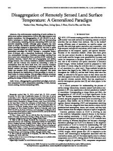
Figure Surface Temperature product on 3on April 20152015 (01:30 PM) PM) that Figure 1. 1. An An example exampleofofthe theMODIS MODISLand Land Surface Temperature product 3 April (01:30 demonstrates cloudcloud obstruction (e.g., WA, and ACT) whichwhich affectsaffects the availability of thisofLand that demonstrates obstruction (e.g., SA, WA,NSW SA, NSW and ACT) the availability this Surface Temperature product. Note that the gray shading is an area that was not observed by the MODIS Land Surface Temperature product. Note that the gray shading is an area that was not observed by the sensor onsensor that particular day. Also, this thepresents abbreviations for the Australian states that will MODIS on that particular day.figure Also,presents this figure the abbreviations for the Australian be further reference purposes. states thatused will for be further used for reference purposes.
As an example, operational flood warning systems are driven by precipitation as the main predictor and the initial (wetness) conditions of the land surface needs to be determined through various sources of remote sensing information [4]. Specifically for a warning system, cloud obstruction is a major limitation of TIR observations due to the strong link between clouds and precipitation generally leading to the absence of thermal infrared (TIR) observations in those final
Remote Sens. 2016, 8, 162
3 of 14
As an example, operational flood warning systems are driven by precipitation as the main predictor and the initial (wetness) conditions of the land surface needs to be determined through various sources of remote sensing information [4]. Specifically for a warning system, cloud obstruction is a major limitation of TIR observations due to the strong link between clouds and precipitation generally leading to the absence of thermal infrared (TIR) observations in those final days leading up to an actual inundation event. In order to overcome this limitation within a critical time period, we aim to develop a relatively simple merging scheme that can benefit from the advantages of both TIR and passive microwave observations. 2. Land Surface Temperature Data Several LST products were used in this study including two products obtained by space-borne remote sensing and an output of a re-analysis model to particularly increase our understanding over the various climate zones that Australia contains. The primary LST source comes from the MODIS sensor (Section 2.1) onboard the NASA Aqua satellite. The second LST data product comes from the multi frequency passive microwave sensor onboard the Japanese Aerospace eXploration Agency (JAXA) Global Chance Observation Mission-Water (GCOM-W) satellite (Section 2.2) and the re-analysis LST data product from Modern Era Retrospective-analysis for Research and Applications (MERRA; Section 2.3) which was primarily used for independent comparison purposes in this study and serves as a consistent reference to better understand spatial patterns over the entire country, particularly over the climate zones. 2.1. MODIS Both NASA’s Terra and Aqua satellites carry MODIS sensors and were launched in 1999 and 2002, respectively. In this study, we use the LST product obtained from the MODIS sensor onboard the Aqua satellite as its local equatorial overpass time coincides with that of the GCOM-W satellite. Both (Aqua and GCOM-W) have their day time equatorial overpass around 1.30 PM (ascending) and their night time overpass around 1.30 AM (descending). The MODIS LST is at a high spatial resolution (around 1 km) compared to passive microwaves (around 10 km), however, in this study we used the MYD11C1 (MODIS Aqua) product of which the standard product is aggregated into 0.05˝ grid boxes. This product was further aggregated into 0.10˝ grid boxes to spatially match the microwave observations. The MODIS LST product is retrieved through the split window method [5] that uses TIR channels 31 and 32. This MODIS LST product has been extensively validated against ground based observations (e.g., [6–8]) and radiance based validation studies. Relevant for the current study is that [7] showed the high consistency between TIR- and microwave- based LST products against ground observations over a number of sites located in the Murrumbidge catchment located in Southeast Australia, hence demonstrating the high potential for combining those remotely sensed products. In this study, the MYD11C1 LST product was further aggregated into 0.10˝ grid boxes to get a spatial match with the LST product derived from the Advanced Microwave Scanning Radiometer 2 (AMSR2) sensor on GCOM-W. For consistency reasons in the analyses, we only included aggregated MODIS LST data product in absence of any cloud and aerosol contamination. Furthermore, unless mentioned otherwise, a 3-year period was analyzed starting on 24 July 2012, coinciding with the start of the operational status of AMSR2, to the same calendar day in 2015. The MODIS MYD11C1 LST data was provided by the United States Geological Survey [5]. 2.2. AMSR2 The AMSR2 is a multi-frequency passive microwave sensor onboard JAXA’s GCOM-W satellite. This satellite was launched on 17 May 2012 and is the first in a series that is expected to contribute to observing various aspects of the carbon and hydrological cycle including precipitation, water vapor, soil moisture, snow depths, carbon, radiation and sea water temperature. Passive microwave
Remote Sens. 2016, 8, 162
4 of 14
observations are sensitive to the land surface and water and, therefore, play an important role in observing the varying phases and quantities of water in both time and space. AMSR2 is the successor of the successful Advanced Microwave Scanning Radiometer for Earth Observing Systems (AMSR-E) that provided Earth scientists an almost decadal, consistent and continuous global passive microwave database. AMSR2 and AMSR-E have an almost identical sensor setup that covers a range of microwave frequencies, although AMSR2 was further improved based on the extensive experience with its predecessor. The spatial resolution, spectral resolution and sensor accuracies of AMSR2 were all improved and an additional C-band channel (7.3 GHz) was successfully added to mitigate artificial radio frequency interference [9]. Several approaches that link passive microwave observations to LST were developed over the recent years. Holmes et al. 2009 [10] presents a simple, general approach and compared its performance at the global scale by extensive validation against flux tower data and also provided a global comparison against modelled data. They presented an approach that related the vertically polarized Ka-band frequency channel (Tb, 37V ) to LST through a single linear regression model with global applicability. Based on comparison against in situ observations, Holmes et al. 2009 [10] determined a threshold of 259.8 K for its global regression model—transition point under which passive microwave emissions behaves nonlinearly. Over Australia, their error simulations suggested relatively small biases generally ranging between 1.5 and ´1.5 degrees [K] with the exception of the Simpson Desert located in Central Australia. In the present study, the single regression model to derive LST globally was used as described in Section 3.1, and compared against an existing LST product. In the next scaling step, a linear regression model was adopted and applied at individual pixel level as detailed in Section 3.2. 2.3. MERRA MERRA provides a global re-analysis data record to support earth science objectives of NASA with a special emphasis on the global hydrological cycle [11]. Several diagnostics are produced at 6-hourly intervals whereas others, including LST, are produced at hourly intervals. The MERRA data product comes in a relatively coarse spatial resolution of 1/2˝ latitude by 2/3˝ longitude. In this study, MERRA serves as a consistent reference that could provide additional quality information about the individual and merged LST products. Additionally, our main interest is over large areas so Australia was subdivided into major climate zones. MERRA was used consistently over these different zones as ground based observations in isolated monitoring networks lack spatial consistency over large spatial domains [12]. This particular purpose justifies a nearest neighbor re-sampling of this coarse product to a finer grid that matches the AMSR2 observations as well as the aggregated MODIS observations. MERRA data is publically available through the Goddard Earth Sciences Data and Information Services Centre; for more information on the MERRA data, readers are directed to [11]. 3. Methodology and Results In the first step, the existing remotely sensed LST products are compared over Australia to gain a better understanding of their differences and similarities. Our analysis is focused on the temporal agreement as systematic differences may exist due to the different vertical depths that are observed; [7] hence, coefficient of determination (R2 ) and standard error (SE) are the metrics of interest. This SE was determined through Equation (1) in which σx represents the variation in the MODIS LST. In order to better understand seasonal trends and interannual variability, this part of the analysis was done on both anomalies after removing the climatology as well as raw timeseries. The decomposition into anomalies was done through a standard approach that uses a 31-day moving window centered on a particular day of the year following [4]. In the next step, the scalability of the passive microwave based product is examined and a relatively simple merging approach was proposed. Then, the various different LST products and the combined product were compared against the MERRA re-analysis LST dataset that serves as a consistent reference over the various climate zones that Australia experiences,
Remote Sens. 2016, 8, 162
5 of 14
again for anomalies and raw timeseries. Finally, the comparison against MERRA was divided over these four major climate zones to further understand their agreement. SE “ σx
a 1 ´ R2
(1)
3.1. Comparing Existing Products A direct comparison between the LST products from MODIS and AMSR2 was presented in order to better understand their potential differences and similarities. Figure 2 was based on the anomalies Remote Sens. 2016, 8, 162 5 of 13 and presents both the R2 (left) and the SE (right) for the observations that were taken during the 2 (left)(bottom). day (top) and during the Rnight rawfortime series were analyzed in anduring identical and presents both the and the SEThe (right) the observations that were taken the way day and those(top) spatial presented theraw supplementary material S1). Furthermore, and maps duringwere the night (bottom).inThe time series were analyzed(Figure in an identical way and thosethese spatial maps were presentedseparated in the supplementary material S1).physical Furthermore, these satellite satellite paths were explicitly to understand how(Figure different conditions during the paths were explicitly separated to understand how different physical conditions during the day and day and the night impact these LST products. A common assumption (e.g., [13,14]) in applications the night impact these LST products. A common assumption (e.g., [13,14]) in applications that that use LST products is that the soil and canopy temperature are equal during the nightuse due to LST products is that the soil and canopy temperature are equal during the night due to thermal thermal equilibrium. During the day, this assumption introduces uncertainties due to the imposed equilibrium. During the day, this assumption introduces uncertainties due to the imposed cooling cooling effect of transpiration which generally results in soil temperatures that are higher than canopy effect of transpiration which generally results in soil temperatures that are higher than canopy temperatures. This This phenomenon maymay impact the products differently as theasoriginal spatialspatial resolution temperatures. phenomenon impact the products differently the original of theresolution MODIS of LST is 1product km; hence, thishence, product may have ability to represent canopy theproduct MODIS LST is 1 km; this product maybetter have better ability to represent and soil temperature separatelyseparately than the passive LST product. canopy and soil temperature than the microwave passive microwave LST product.
Figure 2. high The high agreement between the anomalies Surface Temperature products from Figure 2. The agreement between the anomalies LandLand Surface Temperature products from MODIS 2 (a) for day time observations; SE (b) for day time observations; 2 MODIS and AMSR2 expressed in R and AMSR2 expressed in R (a) for day time observations; SE (b) for day time observations; R2 (c) for 2 (c) for night time observations and SE (d) for night time observations. nightRtime observations and SE (d) for night time observations.
For the anomalies, it was found that the mean R2 values over Australia were high for both the For anomalies, it was found the meanThe R2 values Australia were high forfrom both the day the (R2 0.48) and night (R2 0.56) timethat observations. mean R2over values for the raw time series 2 2 2 day (R 0.48) time observations. meanand R2 night values thetime rawobservations. time series from Figure S1and werenight found(Rto 0.56) be even higher, for the dayThe (R 0.82) (R2for 0.85) 2 0.82)similarities The distribution of these R2 values showed for The Figure S1spatial were found to be even higher, for the day (Rmany and nightbut (R2also 0.85)some timedifferences observations. 2 both the day and night time observations, as well as the anomalies compared to the raw time series. spatial distribution of these R values showed many similarities but also some differences for both the Generally, the products show very high agreement with R2 ranging from 0.75time for the anomalies day and night time observations, as well as the anomalies compared to0.50 theto raw series. Generally, and from 0.8 to 1.0 for the raw time series over2the central part of Australia. This agreement tends to the products show very high agreement with R ranging from 0.50 to 0.75 for the anomalies and from drop in the tropical regions located in the north of Australia with relatively low agreement in the far 0.8 to 1.0 for the raw time series over the central part of Australia. This agreement tends to drop in the north of WA and the Northern Territory (NT) for the day time observations and a relatively low tropical regionsinlocated in theofnorth of Australia agreementAnother in the far north of WA agreement the far north Queensland (QLD) with for therelatively night timelow observations. feature that and the Northern Territory (NT) foreffect the day and on a relatively low agreement stands out in the R2 maps is the thattime openobservations water may have the agreement between thein the far north of Queensland the night time observations. Another feature that outinin the products, which tends(QLD) to dropfor significantly as shown for Lake Eyre, Lake Torrens, Lakestands Gairdner 2 resultstends R2 maps is the effect that and open water maythat have on the products, SA, and Lake Mackay Lake Argyle border WAagreement and the NT.between Inversely,the this drop in Rwhich in an increase in SE over these lakes and is evident in both the anomalies and raw time series as well as the different overpasses. Another feature that stands out in the SE maps is the contrast between the day and the night time maps which are reflected in the higher mean values over Australia for the day (SE 3.18 K for the anomalies) as compared to night (SE 1.88 K for the anomalies) time observations. This contrast is in agreement with the commonly used assumption (e.g., [13,14]) that was previously mentioned.
Remote Sens. 2016, 8, 162
6 of 14
to drop significantly as shown for Lake Eyre, Lake Torrens, Lake Gairdner in SA, and Lake Mackay and Lake Argyle that border WA and the NT. Inversely, this drop in R2 results in an increase in SE over these lakes and is evident in both the anomalies and raw time series as well as the different overpasses. Another feature that stands out in the SE maps is the contrast between the day and the night time maps which are reflected in the higher mean values over Australia for the day (SE 3.18 K for the anomalies) as compared to night (SE 1.88 K for the anomalies) time observations. This contrast is in agreement with the commonly used assumption (e.g., [13,14]) that was previously mentioned. Remote Sens. 2016, 8, 162 6 of 13 In order to further understand the comparison between both LST products, histograms that portray the relative frequency of these two metrics were also presented in a similar order as Figure 2. In order to further understand the comparison between both LST products, histograms that Figure 3 presents the distribution R2 and SE for were the anomalies whereas the histograms of the portray the relative frequency ofof these two metrics also presented in a similar order as Figure 2. raw time series presented in in the of supplementary material (Figure S2).theThese histograms confirm Figure were 3 presents the distribution R2 and SE for the anomalies whereas histograms of the raw that the majority of R2 over is withinmaterial the high rangeS2). that washistograms indicatedconfirm earlier and timevast series were presented in inAustralia the supplementary (Figure These that the vast majority R2 over Australia within the high range that was indicated earlier also and that that only a fraction of theofanalyzed pixels is show a weak agreement. These histograms confirm only a fraction of the analyzed pixels show a weak agreement. These histograms also confirm the SE the contrasting agreement between the day and night-time observations with significantly lower contrasting agreement between the day and night-time observations with significantly lower SE and values for the night time LST products. The relative differences in the histograms of the anomalies values for the night time LST products. The relative differences in the histograms of the anomalies the raw time series are also in line with expectations, particularly the overall drop in R2 shifting the and the raw time series are also in line with expectations, particularly the overall drop in R2 shifting entire histogram to a lower range. Again, the day and night-time contrast is in agreement with earlier the entire histogram to a lower range. Again, the day and night-time contrast is in agreement with findings (e.g., [13,14]) on thermal equilibrium. earlier findings (e.g., [13,14]) on thermal equilibrium.
Figure 3. Histograms of the anomalies that show the agreement between the Land Surface
Figure 3. Histograms of the anomalies that show the agreement between the Land Surface Temperature Temperature products from MODIS and AMSR2 expressed in R2 (a) for day time observations, SE (b) 2 (a) for day products from MODIS and AMSR2 expressed in R time observations, SE (b) for day time for day time observations, R2 (c) for night time observations and SE (d) for night time observations. 2 observations, R (c) for night time observations and SE (d) for night time observations.
As previously mentioned (Section 2.2), the original passive microwave LST algorithm used a predetermined to (Section delineate 2.2), frozen unfrozen conditions. A simple wasused As previously threshold mentioned theand original passive microwave LSTanalysis algorithm conducted in order to determine the effect of suchand nonlinearities our study A area. The analysis as was a predetermined threshold to delineate frozen unfrozen over conditions. simple analysis presented in Figure 2 was repeated without the implementation of this predetermined threshold for conducted in order to determine the effect of such nonlinearities over our study area. The analysis both the anomalies and raw time series. These results confirm the nonlinear behavior below this as presented in Figure 22 was repeated without the implementation of this predetermined threshold preset threshold as R drops and SE increases in absence of the masking procedure which was shown for both the anomalies and raw time series. These results confirm the nonlinear behavior below to be consistent for day- and night-time observations (Table 1). However, this analysis also shows its 2 drops and SE increases in absence of the masking procedure which was this preset threshold as Rour marginal impact over study area as R2 is marginally higher and SE is marginally lower with the shown to be consistent for dayand night-time observations 1). of However, thisprocedure analysis also masking procedure applied. Finally, a note should be made that (Table the impact this masking 2 shows marginal impactrather oversignificant our studyinarea as Rwith is marginally higherfreezing and SEseasons is marginally is its expected to become regions more pronounced than thatlower of Australia. with the masking procedure applied. Finally, a note should be made that the impact of this masking
procedure is expected to become rather significant in regions with more pronounced freezing seasons Table 1. Mean R2 and SE over Australia that demonstrates the impact of a routinely applied masking than that of Australia. procedure over our study area. Note that the statistics for the anomalies were presented first and those for the raw timeseries were presented within brackets.
R2 SE
Night Time Observations No Masking Tb, 37V < 259.8 Masked 0.561 (0.844) 0.563 (0.847) 1.888 (2.012) 1.885 (2.000)
Day Time Observations No Masking Tb, 37V < 259.8 Masked 0.478 (0.818) 0.480 (0.819) 3.189 (3.461) 3.183 (3.451)
Remote Sens. 2016, 8, 162
7 of 14
Table 1. Mean R2 and SE over Australia that demonstrates the impact of a routinely applied masking procedure over our study area. Note that the statistics for the anomalies were presented first and those for the raw timeseries were presented within brackets. Night Time Observations R2 SE
Day Time Observations
No Masking
Tb, 37V < 259.8 Masked
No Masking
Tb, 37V < 259.8 Masked
0.561 (0.844) 1.888 (2.012)
0.563 (0.847) 1.885 (2.000)
0.478 (0.818) 3.189 (3.461)
0.480 (0.819) 3.183 (3.451)
3.2. Linear Scaling of Microwave Observations In this section, a relatively simple scaling approach is proposed which is very much in line with the Remote Sens. 2016, 8, 162 7 of 13 general solution presented by [10] but with the explicit goal to scale the AMSR2 (Tb, 37V ) observations in the MODIS LST product. The logic behind this experimental setup is that (1) Microwave based 3.2. Linear Scaling of Microwave Observations LST is considered to be an alternative to based LST and (2) MODIS has the capabilities to observe In this section, a relatively simpleTIR scaling approach is proposed which is very much in line with at higherthe spatial resolution (up to 1 km). These two factors justify to AMSR2 treat MODIS general solution presented by [10] but with the explicit goalthe to choice scale the (Tb, 37V) LST as observations MODISalways LST product. The logic this experimental setup is higher that (1) spatial the primary productinasthe it would be preferred in behind operational schemes due to its Microwave based LST is considered that to bethe an alternative to TIR of based LST and (2) MODIS has the resolution. We should again emphasize main predictor flooding—that is, precipitation—is capabilities to observe at higher spatial resolution (up to 1 km). These two factors justify the choice generally associated with cloud cover leading to the absence of thermal infrared (TIR) observations to treat MODIS LST as the primary product as it would always be preferred in operational schemes due towards the most critical time period in a flood warning system. A pixel based linear regression was to its higher spatial resolution. We should again emphasize that the main predictor of flooding—that executedis,for MODIS LSTgenerally and AMSR2 (Tb,with observations, thetodayand night-time observations 37V )cloud precipitation—is associated cover leading the absence of thermal infrared were again analyzed Thetime slope andinoffsets only determined for the raw (TIR)explicitly observations towardsseparately. the most critical period a floodwere warning system. A pixel based linear regression was executed for anomalies MODIS LST and AMSR2 in (Tb,a37Vfollow ) observations, theFigure day- and nighttimeseries as the decomposition into is applied on step. 4 presents the time observations were again explicitly analyzed separately. The slope and offsets were only slope values (left) of the pixel based linear regression and the corresponding offset values (middle) determined for the raw timeseries as the decomposition into anomalies is applied in a follow on step. were also reported. Additionally, we also presented the sample sizes (right) within the three year Figure 4 presents the slope values (left) of the pixel based linear regression and the corresponding analysisoffset period used to determine the regression parameters. The spatial pattern of these sample values (middle) were also reported. Additionally, we also presented the sample sizes (right) sizes is awithin directthefunction the (remotely sensed) revised times combined with (natural) three yearofanalysis period used to determine the regression parameters. Thethe spatial pattern spatial variability of cloud cover Again, observations that were taken thewith day the (top) and of these sample sizesand is aaerosols. direct function of the (remotely sensed) revised timesduring combined (natural) spatial variability of cloud cover and aerosols. Again, observations that were taken during during the night (bottom) were separated. In this pixel based regression analysis, there is dependence day and (top) offset and during the which night (bottom) were separated. In this pixel based regression analysis, betweenthe slope values result in distinct spatial patterns. Many regions, such as the there is dependence between slope and offset values which result in distinct spatial patterns. Many Tropical regions located in the north of Australia and the large lakes in WA, SA and the NT therefore regions, such as the Tropical regions located in the north of Australia and the large lakes in WA, SA show a distinct spatial pattern both the slope and offset. and the NT therefore showina distinct spatial pattern in both the slope and offset.
Figure 4. Pixel based scaling parameters (slope and offset) for MODIS Land Surface Temperature and
Figure 4.AMSR2 Pixel based parameters (slope MODIS Temperature observations. The slope (a); and offsetoffset) (b) andforthe sample Land sizes Surface (c) for day-time (Tb, 37V) scaling and AMSR2 (Tb, 37Vand ) observations. The(e)slope (a); offset (b)(f)and the sample sizes (c) for day-time observations the slope (d); offset and the sample sizes for night-time observations. observations and the slope (d); offset (e) and the sample sizes (f) for night-time observations. 3.3. A Comparison against MERRA The pixels based slope and offset presented in Figure 4 were now used to scale AMSR2 (Tb, 37V) observations into the MODIS LST product through Equation (2). Each individual pixel in time was assessed and gaps in the MODIS LST product that were caused by clouds or aerosols were, in case AMSR2 observations were available, filled through the pixels based linear regression (Equation (2)). =
,
(2)
Remote Sens. 2016, 8, 162
8 of 14
3.3. A Comparison against MERRA The pixels based slope and offset presented in Figure 4 were now used to scale AMSR2 (Tb, 37V ) observations into the MODIS LST product through Equation (2). Each individual pixel in time was assessed and gaps in the MODIS LST product that were caused by clouds or aerosols were, in case AMSR2 observations were available, filled through the pixels based linear regression (Equation (2)). LSTGap f illed “ slope ˆ Tb,37v ` o f f set Remote Sens. 2016, 8, 162
(2) 8 of 13
These combined MODIS and AMSR2 time series were also deseasonalized resulting in anomalies from the combined LST product. Hence, the combined LST product benefits from the cloud penetrating These combined MODIS and AMSR2 time series were also deseasonalized resulting in anomalies from the microwaves combined LSTobservations product. Hence, the combined LST product benefits from thecompared cloud capacity of the passive leading to an increased revisit frequency passive microwaves observationsMODIS leadingand to an increased revisitwere to thepenetrating individual capacity MODIS of LSTtheproducts. Here, both individual AMSR2 products frequency compared to the individual MODIS LST products. Here, both individual MODIS and the compared against the MERRA re-analysis data as well as the combined LST products in which AMSR2 products were compared against the MERRA re-analysis data as well as the combined LST scaled AMSR2 observations fill the cloud gaps in MODIS. The results from this comparison were products in which the scaled AMSR2 observations fill the cloud gaps in MODIS. The results from this presented in Figure 5, which shows the R2 of the three different product combinations and the comparison were presented in Figure 5, which shows the R2 of the three different product combinations percentage of observations that was gained through the addition of the passive microwaves for the and the percentage of observations that was gained through the addition of the passive microwaves for night-time observations alone. This comparison against MERRA was repeated for the raw time series the night-time observations alone. This comparison against MERRA was repeated for the raw time series of which the results were presented material(Figure (Figure of which the results were presentedininthe thesupplementary supplementary material S3).S3).
Figure 5. R2 between the anomalies from MERRA and (a) MODIS; (b) the merged MODIS-AMSR2
2 between the anomalies from MERRA and (a) MODIS; (b) the merged MODIS-AMSR2 FigureLand 5. RSurface Temperature product and (c) AMSR2, as well as the percentage of gained samples Land Surface (c) AMSR2, through Temperature the addition ofproduct AMSR2 and observations (d). as well as the percentage of gained samples through the addition of AMSR2 observations (d). The individual MODIS (Figure 5a) and the AMSR2 LST products (Figure 5c) show a very similar agreement against the independent MERRA dataset with relative high R2 values overa very the vast The individual MODIS (Figure 5a) and the AMSR2 LST products (Figure 5c) show similar majority of central Australia for both the anomalies and raw time series. When comparing results 2 agreement against the independent MERRA dataset with relative high R values over the vast majority from the anomalies (Figure 5) against the raw time series (Figure S3), there is a tendency of lower R2 of central Australia for both the anomalies and raw time series. When comparing results from the values for the anomalies. This lower agreement is the result of removing seasonal trends hence anomalies (Figurethe 5) against time series (Figure S3), there is a tendency of lower R2 values representing skills of the the raw various products to represent the interannual variability. It should for thefurthermore anomalies.be This lower is the result removing seasonal trends hence generally representing noted thatagreement such a drop is in line of with expectations [4] as anomalies the skills of the various products to represent the interannual variability. It should furthermore demonstrate lower agreement than raw time series. The agreement between the MODIS and AMSR2 be dataset breaks in the[4] Tropical climate zone locateddemonstrate in the north of notedLST thatproducts such a and dropthe is MERRA in line with expectations as anomalies generally lower Australia this is more profound for AMSR2between than it isthe forMODIS MODIS. and In this part ofLST Australia, it is and agreement thanand raw time series. The agreement AMSR2 products likely difficult observeinLST passive microwaves due to clouds and active the MERRA datasettobreaks thethrough Tropical climate zone located inrain the bearing north of Australia and this precipitation but land surface modelling may also suffer larger uncertainties due to convection is more profound for AMSR2 than it is for MODIS. In this part of Australia, it is likely difficult to processes [15]. Likewise, this agreement breaks for both products in Southern Victoria (VIC) and Tasmania (TAS). On the other hand, decreasing agreement between MODIS and MERRA was shown in the southern part of WA whereas AMSR2 shows moderate agreement with MERRA in these regions. Generally, the agreement between MERRA and MODIS (Figure 5a) is highest with a country average R2 of 0.26 for anomalies and R2 of 0.76 for raw time series followed by the AMSR2 product (R2 0.16 for anomalies and R2 0.66 for raw time series) and the combined product (R2 0.18 for
Remote Sens. 2016, 8, 162
9 of 14
observe LST through passive microwaves due to rain bearing clouds and active precipitation but land surface modelling may also suffer larger uncertainties due to convection processes [15]. Likewise, this agreement breaks for both products in Southern Victoria (VIC) and Tasmania (TAS). On the other hand, decreasing agreement between MODIS and MERRA was shown in the southern part of WA whereas AMSR2 shows moderate agreement with MERRA in these regions. Generally, the agreement between MERRA and MODIS (Figure 5a) is highest with a country average R2 of 0.26 for anomalies and R2 of 0.76 for raw time series followed by the AMSR2 product (R2 0.16 for anomalies and R2 0.66 for raw time series) and the combined product (R2 0.18 for anomalies and R2 0.62 for raw time series). Remote Sens. 2016, 8, 162 9 of 13 Figure 6 present histograms of the results of this comparison against MERRA, again for the individual MODIS LST product (Figure 6a), the AMSR2 LST product (Figure 6b) and the combined LST product comparison against MERRA, again for the individual MODIS LST product (Figure 6a), the AMSR2 Remote 2016, 8, 162 of 13 (Figure 6c).Sens. This comparison was repeated for the raw timeseries of which the results were 9presented LST product (Figure 6b) and the combined LST product (Figure 6c). This comparison was repeated for in thethe supplementary material (Figure S4). raw timeseries of which the results were presented in the supplementary material (Figure S4). comparison against MERRA, again for the individual MODIS LST product (Figure 6a), the AMSR2 LST product (Figure 6b) and the combined LST product (Figure 6c). This comparison was repeated for the raw timeseries of which the results were presented in the supplementary material (Figure S4).
Figure 6. Histograms that showthe theagreement agreement between between the from MERRA LandLand Surface Figure 6. Histograms that show theanomalies anomalies from MERRA Surface Temperature and the remotely sensed Land Surface Temperature products from MODIS (a); AMSR2 Temperature and the remotely sensed Land Surface Temperature products from MODIS (a); AMSR2 (b) and through the presented combination approach (c) expressed in R2. 2 Figure 6. Histograms that show the agreement between the anomalies (b) and through the presented combination approach (c) expressed in Rfrom . MERRA Land Surface Temperature and the remotely sensed Land Surface Temperature products from MODIS (a); AMSR2 These results were furthermore divided in the different Köppen-Geiger climate zones [16] that (b) and through the presented combination approach (c) expressed in R2.
These results were furthermore divided in Köppen-Geiger climate zones [16] that Australia experiences, the spatial distribution of the thesedifferent climate zones was presented in Figure 7. These different zones are based on the original Köppen classification which was modified by [16] and Australia These experiences, the spatial distribution climateKöppen-Geiger zones was presented in Figure 7. These results were furthermore divided of in these the different climate zones [16] that consists of 29 different climate sub categories globally and 12 sub categories for Australia. These 12 different zones are based on the original Köppen classification which was modified by [16] and consists Australia experiences, the spatial distribution of these climate zones was presented in Figure 7. These Australian sub categories were divided into four major climate zones including tropical, arid desert, of 29 different differentzones climate categories globallyKöppen and 12 classification sub categories for Australia. These Australian aresub based on the original which was modified by 12 [16] and arid steppe and temperate. Three categories were and merged in the tropicalfor (A) climate zone and consists of were 29 different climate subsub categories globally 12 sub categories Australia. These sub categories divided into four major climate zones including tropical, arid desert, arid12 steppe they include rainforest (f), monsoon (m) and Savannah (w). Furthermore, the arid desert (BW) and Australian sub categories were divided into four major climate zones including aridthey desert, and temperate. Three sub categories were merged in the tropical (A) climatetropical, zone and include arid steppe (BS) were separated into a major climate zone and both consist of two different sub arid steppe and temperate. Three sub categories were merged the desert tropical(BW) (A) climate zone and (BS) rainforest (f), monsoon (m) and Savannah Furthermore, theinclimate arid andfive arid steppe categories including hot(f), (h)monsoon and cold(m) (k).(w). Finally, the temperate zone different they include rainforest and Savannah (w). Furthermore, theincludes arid desert (BW) and were sub separated into a major climate andthat bothwere consist of two different sub categories including hot (Csa, Csb, Cwa, Cfazone and aCfb) categorized on drought anddifferent temperature aridcategories steppe (BS) were separated into major climate zone and based both consist of two sub (h) and cold (k). Finally, the temperate climate zone includes five different sub categories (Csa, Csb, indicators throughout the(h) season. Figure presents the spatial extent of these Köppen-Geiger sub categories including hot and cold (k).7Finally, the temperate climate zone 12 includes five different Cwa,sub Cfacategories and Cfb) that were categorized based on drought and temperature indicators throughout the categories over(Csa, Australia including the four major climate zones that were further used in this study. Csb, Cwa, Cfa and Cfb) that were categorized based on drought and temperature season. Figure 7 presents the spatial extent of these 12 Köppen-Geiger sub categories over Australia indicators throughout the season. Figure 7 presents the spatial extent of these 12 Köppen-Geiger sub including the four climate zones this study. categories over major Australia including thethat fourwere majorfurther climateused zonesin that were further used in this study.
Figure 7. Australia’s major climate zones according to the Köppen-Geiger climate classification. Several sub categories of the more detailed classification were merged into these four major classes. Figure 7. Australia’s major climate zones according to the Köppen-Geiger climate classification.
Figure 7. Australia’s climate zones according to climate the Köppen-Geiger climate classification. Several Table 2 providesmajor the averaged results per major zone and demonstrates a high degree of Several sub categories of the more detailed classification were merged into these four major classes. consistency compared to the country average results both the theclasses. raw time series. sub categories of the more detailed classification werefor merged intoanomalies these fourand major First,Table the relative agreement between MERRA both individual anddemonstrates merged products is consistent 2 provides the averaged results per and major climate zone and a high degree of with highest agreement for MODIS and the lowest agreement for the combined product, consistency compared to the country average results for both the anomalies and the raw time series. demonstrated by both R2 and SE metrics. The lowest agreement for all products was generally found First, the relative agreement between MERRA and both individual and merged products is consistent in the highest tropical agreement climate zone the the temperate zone, for aridthe steppe and theproduct, highest with forfollowed MODISbyand lowestclimate agreement combined agreement was found over arid deserts. It should be emphasized that the agreement drops the demonstrated by both R2 and SE metrics. The lowest agreement for all products was generallyfor found merged product comes with a significant increase (20% on average) in number of observations gained
Remote Sens. 2016, 8, 162 Remote Sens. 2016, 8, 162
10 of 14 10 of 13
in percentage, which is effectively combination mapclimate between revised time of the individual sensors Table 2 provides the averagedaresults per major zone and demonstrates a high degree of and cloud contamination. Thecountry central part of the country gains 10%–20% more consistency compared to the average results for generally both the anomalies and the rawobservations time series. but some regions, such as between TAS, southern Tropicaland regions located in the north of First, the relative agreement MERRAVIC andand boththe individual merged products is consistent Australia, generally gainfor more thanand 30%the more observations. is concluded that the significant with highest agreement MODIS lowest agreementHence, for the itcombined product, demonstrated gain in observations through thelowest MODIS-AMSR2 comes that penalty inin performance. by both R2 and SE metrics. The agreement combinations for all products was at generally found the tropical
Night Time
climate zone followed by the temperate climate zone, arid steppe and the highest agreement was found 2. Summarized for the MERRA the the individual and over Table arid deserts. It shouldstatistics be emphasized that thecomparison agreementagainst drops for mergedMODIS product comes AMSR2 LST products and the combined product in which cloud gaps in MODIS were filled with with a significant increase (20% on average) in number of observations gained by adding AMSR2 AMSR2 observations. Note that the statistics for the anomalies were presented first and those to thescaled individual MODIS based product. Figure 5d expresses this observation gain in percentage, for the raw timeseries were presented within brackets. which is effectively a combination map between revised time of the individual sensors and cloud contamination. The central part of the country generallyClimate gains 10%–20% more observations but some Zone MERRA Arid Desert located Arid regions, such as TAS, southern VICTropical and the Tropical regions in Steppe the north of Temperate Australia, generally R2 SE SE that R2the significant SE R2 in observations SE gain more than 30% more observations. Hence, it Ris2 concluded gain 0.20 2.17 0.30 2.59 0.27 2.55 0.16 2.68 through the MODIS-AMSR2 combinations comes at that penalty in performance. MODIS
Day Time
(0.56) (2.52) (0.84) (2.74) (0.77) (2.78) (0.64) (2.85) 0.12 3.29 0.19 3.21 0.16 3.30 0.11 Table 2. Summarized statistics for the MERRA comparison against the individual MODIS and3.25 AMSR2 AMSR2 (0.36) (2.76) (0.73) (3.41)in MODIS (0.64) were (3.34) (0.62) LST products and the combined product in which cloud gaps filled with scaled(2.73) AMSR2 0.11 2.80the anomalies 0.22 3.12 0.19 3.11 and those 0.13 for 2.80 observations. Note that the statistics for were presented first the raw MODIS-AMSR2 (0.30)brackets. (3.39) (0.71) (3.66) (0.61) (3.64) (0.55) (3.21) timeseries were presented within 0.09 4.02 0.33 3.63 0.30 3.95 0.39 3.52 MODIS (0.50) (4.35) (0.83) (4.19) (4.33) (0.81) (3.84) Climate(0.74) Zone 0.22 4.11 0.39 4.11 0.38 4.10 0.43 3.73 MERRA Tropical Arid Desert Arid Steppe Temperate AMSR2 (0.43) (4.58) (0.76) (5.29) (0.68) (5.13) (0.73) (4.73) SE SE SE SE R2 R2 R2 R2 0.13 4.77 0.32 4.83 0.30 4.92 0.37 4.41 MODIS-AMSR2 0.20 2.17 0.30 2.59 0.27 2.55 0.16 2.68 (0.40) (5.58) (0.71) (6.03) (0.63) (5.93) (0.68) (5.58) MODIS
(0.56) (2.52) (0.84) (2.74) (0.77) (2.78) (0.64) (2.85) 0.12 3.29 0.19 3.21 0.16 3.30 0.11 3.25 (0.36) (2.76) (0.73)merged (3.41) (0.64) (3.34)provides (0.62) in Figure (2.73) 8 and A further example of the individual MODIS and LST products was 0.11 2.80 0.22 0.19 3.11 0.13 was, similar to Figure 1, based on observations made on 33.12 April 2015. Large parts of NSW, 2.80 as well as MODIS-AMSR2 (0.30) (3.39) (0.71) (3.66) (0.61) (3.64) (0.55) (3.21) Night Time
AMSR2
significant parts of northeastern SA, southern QLD and TAS experience cloud cover on this day, 0.09 4.02 0.33 3.63 0.30 3.95 0.39 3.52 MODIS hence the (Figure 8a) presents values in these regions. These cloud (4.35) (0.83)no data (4.19) (0.74) (4.33) (0.81) (3.84) gaps DayMODIS LST product (0.50) 0.22 4.11 0.39 4.11 0.38 4.10 0.43 3.73 Time by AMSR2 were filled AMSR2observations through the proposed combination approach resulting in an (0.43) (4.58) (0.76) (5.29) (0.68) (5.13) (0.73) (4.73) improved coverage over this part (Figure 8b). Figure0.30 8c presents distribution 0.13of Australia 4.77 0.32 4.83 4.92 the spatial 0.37 4.41 MODIS-AMSR2 (5.58) (0.71) (6.03)Regions (0.63)with(5.93) (0.68) are (5.58) of the sensors that were used in(0.40) the combined LST product. gray shading based on MODIS whereas the cyan regions are based on scaled AMSR2 observations.
Figure 8. An example of the individual MODIS LST product for 3 April 2015 (a); the combined Land Figure 8. An example of the individual MODIS LST product for 3 April 2015 (a); the combined Land Surface Temperature product (b) and a spatial map (c) that demonstrates the sensors that were used Surface Temperature product (b) and a spatial map (c) that demonstrates the sensors that were used in in the combined Land Surface Temperature product. The Land Surface Temperature product in the the combined Land Surface Temperature product. The Land Surface Temperature product in the gray gray shading is based on MODIS whereas the cyan regions are based on scaled AMSR2 observations. shading is based on MODIS whereas the cyan regions are based on scaled AMSR2 observations.
Remote Sens. 2016, 8, 162
11 of 14
A further example of the individual MODIS and merged LST products was provides in Figure 8 and was, similar to Figure 1, based on observations made on 3 April 2015. Large parts of NSW, as well as significant parts of northeastern SA, southern QLD and TAS experience cloud cover on this day, hence the MODIS LST product (Figure 8a) presents no data values in these regions. These cloud gaps were filled by AMSR2 observations through the proposed combination approach resulting in an improved coverage over this part of Australia (Figure 8b). Figure 8c presents the spatial distribution of theSens. sensors Remote 2016, that 8, 162were used in the combined LST product. Regions with gray shading are based 11 ofon 13 MODIS whereas the cyan regions are based on scaled AMSR2 observations. A A final final example example that that demonstrates demonstrates the the combination combination approach approach and and its its potential potential usefulness usefulness in in operational operational systems systems was was presented presented in in Figure Figure 9. 9. Australia’s Australia’s central central coast coast received received significant significant amounts amounts of on 21 21 and and 22 22April April2015, 2015,which whichresulted resultedininthe theHunter HunterValley Valley floods and was shown of precipitation precipitation on floods and was shown in in Figure This Figure presentsprecipitation precipitationdata datafor forMaitland, Maitland,aacity citylocated located in in the the Lower Lower Hunter Figure 9. 9. This Figure 9c9cpresents Hunter Valley, for aa five five week week period Valley, for period as as obtained obtained by by the theAustralian AustralianWater WaterAvailability AvailabilityProject Project(AWAP; (AWAP;[17]. [17]. The AWAP precipitation shows roughly three separate precipitation periods of which the first The AWAP precipitation shows roughly three separate precipitation periods of which the first resulted resulted in significant floods. The obvious link between precipitation and obstruction cloud obstruction resulted in significant floods. The obvious link between precipitation and cloud resulted in the in the absence of MODIS data during those precipitation periods. Those gaps in MODIS were then absence of MODIS data during those precipitation periods. Those gaps in MODIS were then filled filled by AMSR2 observations as scaled through the proposed combination approach. The periods by AMSR2 observations as scaled through the proposed combination approach. The periods which which these microwave passive microwave observations were through indicated through a grey heavilyheavily rely on rely theseon passive observations were indicated a grey background background and demonstrate the successful scaling of AMSR2 observations resulting in an increasing and demonstrate the successful scaling of AMSR2 observations resulting in an increasing number of number of LST observations. LST observations.
Figure recent flooding example the Valley Hunter Valley along central Australia’s central coast Figure 9.9.AA recent flooding example for thefor Hunter along Australia’s coast demonstrating demonstrating the combination approach and its usefulness for warning systems. Thissevere area the combination approach and its usefulness for warning systems. This area experienced experienced flooding after receiving amounts precipitation on 21 andtimeseries 22 April flooding aftersevere receiving significant amounts significant of precipitation on 21ofand 22 April 2015. This 2015. This timeseries demonstrates successful scaling resulting of AMSR2 observations resultingof in an demonstrates the successful scaling ofthe AMSR2 observations in an increasing number Land increasing number of Land Surface Temperture observations. (a) LST products during the day; (b) Surface Temperture observations. (a) LST products during the day; (b) LST products during the night; LST products during (c) precipitation from the Australian Water Availability Project. (c) precipitation from the the night; Australian Water Availability Project.
4. Discussion Discussion Areas in which disagreement was found between the MODIS and AMSR2 LST products could partially partially be related to known phenomena and differences between the day and night-time analysis could could be related to the theory of thermal equilibrium. It should be emphasized that precipitation precipitation is generally generally associated associated with with cloud cloud cover cover leading leading to the absence of thermal infrared (TIR) observations towards warning systems, which was thethe initial motivation for towards the the most mostcritical criticaltime timeperiod periodininflood flood warning systems, which was initial motivation aforpixel based scaling approach. The merged MODIS and AMSR2 product revealed a drop a pixel based scaling approach. The merged MODIS and AMSR2 product revealed a drop in performance compared to the individual products, the cost of a gain in revisit times. This performance drop was particularly visible in the tropical climate zone located in the north of Australia and can likely be attributed to higher uncertainties in the passive microwave products due to rain bearing clouds and active precipitation [18], as well as to higher uncertainties in the MERRA land surface model caused by convection processes [15]. Finally, it should be noted that AMSR2 LST
Remote Sens. 2016, 8, 162
12 of 14
performance compared to the individual products, the cost of a gain in revisit times. This performance drop was particularly visible in the tropical climate zone located in the north of Australia and can likely be attributed to higher uncertainties in the passive microwave products due to rain bearing clouds and active precipitation [18], as well as to higher uncertainties in the MERRA land surface model caused by convection processes [15]. Finally, it should be noted that AMSR2 LST retrievals in the merged products were only taken under cloudy conditions. Again, occasional rain bearing clouds or active precipitation may impact microwave emission, particularly when droplets are close to the size of the wavelength [18]. These phenomena could partially explain the performance drop of the merged LST product. In order to further understand the qualities of these individual and merged LST products, further quality assessment is needed. Techniques such as error propagation [19], radiance based validation studies, ground based validation studies or data assimilation techniques could serve as potential tools for this. Additionally, more sophisticated scaling approaches are likely to further improve obtained results as these can account for the impact of nonlinearities. However, it should be emphasized that the relatively simple linear regression performs well over the vast majority of the country. A potential approach to account for nonlinearities could be the replacement of the linear scaling by a polynomial regression approach. However, it should be noted that more sophisticated approaches could potentially hamper its usefulness in near real time application, a major advantage of the relatively simple approach proposed here. 5. Conclusions A relatively simple combination approach that benefits from the cloud penetrating capacity of passive microwaves was presented. In a first step, the MODIS and AMSR2 LST products were compared and very high agreement was found over the vast majority of Australia. This agreement was found for the anomalies resulting in R2 values generally ranging from 0.5 to 0.75 and for raw timeseries resulting in R2 values generally ranging from 0.8 to 1.0. In a next step, pixel based scaling was proposed and the obtained results suggest that passive microwave observations from AMSR2 can successfully fill gaps caused by clouds or aerosol contamination in the MODIS LST product. By using AMSR2, the revised time increased on average by 20% but this varies per pixel as a result of the unique revised times of the satellite sensors as well as cloud and aerosol contamination. It should be emphasized that precipitation is generally associated with cloud cover leading to the absence of thermal infrared (TIR) observations towards the most critical time period in flood warning systems, which is most interesting in operational warning systems. The merged product also revealed a performance drop compared to the individual products which is the cost of a gain in revisit times. This performance drop was particularly visible in the tropical climate zone located in the north of Australia and can likely be attributed to higher uncertainties due to rain bearing clouds and active precipitation [18], as well as to higher uncertainties in the MERRA land surface model caused by convection processes [15]. The comparison against re-analysis data was subdivided over Australia’s major climate zones and revealed that the relative agreement between LST products against the re-analysis data is consistent over all these climate zones. It should be noted that our analysis was done for both raw time series as well as anomalies that better represent the interannual variability of the various products. In line with expectations, the relative performance of the anomalies drops when compared to the raw time series but overall findings were confirmed through both the anomalies and raw time series. Additionally, two examples were provided that demonstrate the proposed merging approach including an example for the Hunter Valley floods along Australia’s central coast that experienced significant flooding in April 2015. Supplementary Materials: The following are available online at www.mdpi.com/http://www.mdpi.com/ 2072-4292/8/2/162, Figure S1: The high agreement between the raw times eries of the Land Surface Temperature products from MODIS and AMSR2 expressed in R2 (a) for day time observations, SE (b) for day time observations, R2 (c) for night time observations and SE (d) for night time observations, Figure S2: Histograms that show the agreement between the raw timeseries of the Land Surface Temperature products from MODIS and AMSR2
Remote Sens. 2016, 8, 162
13 of 14
expressed in R2 (a) for day time observations, SE (b) for day time observations, R2 (c) for night time observations and SE (d) for night time observations, Figure S3: R2 between the raw time series from MERRA and (a) MODIS, (b) the merged MODIS-AMSR2 Land Surface Temperature product and (c) AMSR2, as well as the percentage of gained samples through the addition of AMSR2 observations (d). Note the wider range of the colorbar compared to Figure 5 that presents the results of the anomalies, Figure S4: Histograms that show the agreement between the raw time series from MERRA Land Surface Temperature and the remotely sensed Land Surface Temperature products from MODIS (a), AMSR2 (b) and through the presented combination approach (c) expressed in R2 . Acknowledgments: This work has been undertaken as part of a Discovery Project (DP140102394) funded by the Australian Research Council. We are grateful to all contributors to the datasets used in this study, particularly we thank the teams from NASA and the Japanese Aerospace Exploration Agency for making their datasets publically available. Author Contributions: R.M. Parinussa initiated the study and did the analysis under the main supervision of A. Sharma. V. Lakshmi and F. Johnson provided regular feedback on the analysis and adviced R.M. Parinussa along the way. All authors contributed to the editing of the manuscript and to the discussion and interpretation of the results. Conflicts of Interest: The authors declare no conflict of interest.
References 1. 2. 3. 4. 5. 6. 7.
8.
9.
10. 11.
12. 13. 14. 15. 16.
Fang, B.; Lakshmi, V.; Bindlish, R.; Jackson, T.; Cosh, M.; Basara, J. Passive microwave soil moisture downscaling using vegetation and surface temperatures. Vadose Zone J. 2013. [CrossRef] Fang, B.; Laskshmi, V. Soil moisture at watershed scale: Remote sensing techniques. J. Hydrol. 2014, 516, 258–272. [CrossRef] Lakshmi, V. A simple surface temperature assimilation scheme for use in land surface models. Water Resour. Res. 2000, 36, 3687–3700. [CrossRef] Parinussa, R.M.; Lakshmi, V.; Johnson, F.M.; Sharma, A. A new framework for monitoring flood inundation using readily available satellite data. Geophys. Res. Lett. 2016. in revision. Wan, Z.; Li, Z.-L. A Physics-based algorithm for retrieving land-surface emissivity and temperature from EOS/MODIS data. IEEE Trans. Geosci. Remote Sens. 1997, 35, 980–996. Bosilovich, M. A comparison of MODIS land surface temperature with in situ observations. Geophys. Res. Lett. 2006, 33, L20112. [CrossRef] Parinussa, R.M.; Jeu, R.; Holmes, T.; Walker, J. Comparison of microwave and infrared land surface temperature products over the NAFE’ 06 research sites. IEEE Geosci. Remote Sens. Lett. 2008, 5, 783–787. [CrossRef] Wan, Z.; Zhang, Y.; Zhang, Q.; Li, Z.-L. Validation of the land surface temperature products retrieved from TERRA moderate resolution imaging spectroradiometer data. Remote Sens. Environ. 2002, 83, 163–180. [CrossRef] De Nijs, A.H.A.; Parinussa, R.M.; Jeu, R.A.M.; Schellekens, J.; Holmes, T.R.H. A methodology to determine radio frequency interference in AMSR2 observations. IEEE Trans. Geosci. Remote Sens. 2015, 53, 5147–5159. [CrossRef] Holmes, T.; Jeu, R.; Owe, M.; Dolman, A. Land surface temperature from Ka-band passive microwave observations. J. Geophys. Res. Atmos. 2009, 114, D04113. [CrossRef] Rienecker, M.; Suarez, M.; Gelaro, R.; Todling, R.; Bacmeister, J.; Liu, E.; Bosilovich, M.; Schubert, S.; Takacs, L.; Kim, G.; et al. MERRA—NASA’s modern-era retrospective analysis for research and applications. J. Clim. 2011, 24, 3624–3648. [CrossRef] Scipal, K.; Holmes, T.R.H.; Jeu, R.A.M.; Naeimi, V.; Wagner, W. A possible solution for the problem of estimating the error structure of global soil moisture datasets. Geophys. Res. Lett. 2008, 35, L24403. [CrossRef] Jeu, R.; Wagner, W.; Holmes, T.; Dolman, A.; Giesen, N.; Friesen, J. Global soil moisture patterns observed by space borne microwave radiometers and scatterometers. Surv. Geophys. 2008, 29, 399–420. [CrossRef] Owe, M.; Jeu, R.; Holmes, T. Multisensor historical climatology of satellite-derived global land surface moisture. J. Geophys. Res. Earth Surf. 2008, 113. [CrossRef] Taylor, C.; Jeu, R.A.M.; Guichard, F.; Haris, P.P.; Dorigo, W.A. Afternoon rain more likely over drier soils. Nature 2012, 489, 423–426. [CrossRef] [PubMed] Peel, M.C.; Finlayson, B.L.; McMahon, T.A. Updated world map of the Köppen-Geiger climate classification. Hydrol. Earth Syst. Sci. 2007, 11, 1633–1644. [CrossRef]
Remote Sens. 2016, 8, 162
17. 18. 19.
14 of 14
Jones, D.; Wang, W.; Fawcett, R. High-quality spatial climate data-sets for Australia. Aust. Meteorol. Oceanogr. J. 2009, 58, 233–248. Ulaby, F.T.; Moore, R.K.; Fung, A.K. Microwave Remote Sensing: Active and Passive; Artech House: Norwood, MA, USA, 1986. Parinussa, R.M.; Meesters, A.; Liu, Y.; Dorigo, W.; Wagner, W.; Jeu, R. Error estimates for near real time satellite soil moisture as derived from the land parameter retrieval model. IEEE Geosci. Remote Sens. Lett. 2011, 8, 779–783. [CrossRef] © 2016 by the authors; licensee MDPI, Basel, Switzerland. This article is an open access article distributed under the terms and conditions of the Creative Commons by Attribution (CC-BY) license (http://creativecommons.org/licenses/by/4.0/).