Comparing Axial CT Slices in Quantized N ... - Semantic Scholar

Comparing Axial CT Slices in Quantized N-dimensional SURF Descriptor Space to Estimate the Visible Body Region Johannes Feulnera,b , S. Kevin Zhouc , Elli Angelopouloua , Sascha Seifertb , Alexander Cavallarod , Joachim Horneggera,e , Dorin Comaniciuc a Pattern

Recognition Lab, Department of Computer Science, Friedrich-Alexander University Erlangen-Nuremberg, Martensstrasse 3, 91058 Erlangen, Germany b Siemens Corporate Technology, G¨ unther-Scharowsky-Str. 1, 91058 Erlangen, Germany c Siemens Corporate Research, Inc., 755 College Road East, Princeton, NJ 08540 d Imaging Science Institute Erlangen, Maximiliansplatz 1, 91054 Erlangen, Germany e Erlangen Graduate School in Advanced Optical Technologies (SAOT), Germany

Abstract In this paper, a method is described to automatically estimate the visible body region of a computed tomography (CT) volume image. In order to quantify the body region, a body coordinate (BC) axis is used that runs in longitudinal direction. Its origin and unit length are patient-specific and depend on anatomical landmarks. The body region of a test volume is estimated by registering it only along the longitudinal axis to a set of reference CT volume images with known body coordinates. During these 1-D registrations, an axial image slice of the test volume is compared to an axial slice of a reference volume by extracting a descriptor from both slices and measuring the similarity of the descriptors. A slice descriptor consists of histograms of visual words. Visual words are code words of a quantized feature space and can be thought of as classes of image patches with similar appearance. A slice descriptor is formed by sampling a slice on a regular 2-D grid and extracting a Speeded Up Robust Features (SURF) descriptor at each sample point. The codebook, or visual vocabulary, is generated in a training step by clustering SURF descriptors. Each SURF descriptor extracted from a slice is classified into the closest visual word (or cluster center) and counted in a histogram. A slice is finally described by a spatial pyramid of such histograms. We introduce an extension of the SURF descriptors to an arbitrary number of dimensions (N-SURF). Here, we make use of 2-SURF and 3-SURF descriptors. Cross-validation on 84 datasets shows the robustness of the results. The body portion can be estimated with an average error of 15.5mm within 9s. Possible applications of this method are automatic labeling of medical image databases and initialization of subsequent image analysis algorithms. Keywords: Body portion estimation, visual words, SURF, N-D

1. Introduction This paper addresses the problem of determining which portion of the body is shown by a stack of axial CT image slices. For example, given a small stack of slices containing the heart region, one may want to automatically determine where in the human body it belongs. Such a technique can be used in various applications such as attaching text labels to images of a database. A user may then search the database for volumes showing the heart. The DICOM protocol already specifies a flag “Body part examined”, but this is imprecise as it only distinguishes 25 body parts. Moreover, the flag can often be wrong as reported by Gueld et al [1]. Or alternatively, our method may be used to reduce traffic load on medical image databases. Often physicians are only interested in a small portion of a large volume stored in the database. If it is known which parts of the body the large image shows, the image slices of interest showing e. g. the heart can be approximately determined and transferred to the user. Another possible application is the pruning of the search space of subsequent image analysis algorithms, like organ detectors. The problem of estimating the body portion of a volume imPreprint submitted to Computerized Medical Imaging and Graphics

age is closely related to inter-subject image registration as it can be solved by registering the volume to an anatomical atlas. This is typically solved in two ways: By detection of anatomical landmarks in the volume image, or by intensity based non-rigid image registration. Landmark based registration may also be used as an initialization for non-rigid registration. However, a set of landmarks is required that covers all regions of the body and can be robustly detected. Intensity based registration tends to be slow, and because it is prone to getting stuck in local optima, it requires a good initialization. In many cases one is only interested in registration along the longitudinal (z) axis and a complete 3-D registration is not necessary. Dicken et al. [2] proposed a method for recognition of body parts covered by CT volumes. An axial slice is described by a Hounsfield histogram with bins adapted to the attenuation coefficient of certain organs. Derived values such as the spatial variance within the slice of voxels of a certain bin are also included into the descriptor. The stack of the N-dimensional axial slice descriptors is interpreted as a set of N 1-D functions whose domain is the (vertical) z level. Then five handcrafted rules are used to decide which of eight different body parts are visible. January 3, 2011

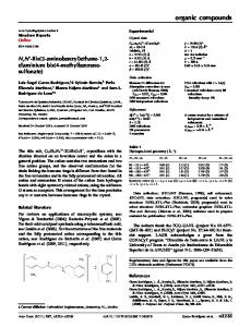
Figure 1: The proposed system for body portion estimation. The axial slices of a CT volume are first processed separately. sample positions are generated on a regular grid. For each sample position inside the patient, a SURF descriptor is computed from the local neighborhood called “patch”. The descriptors are classified into visual words and accumulated in a histogram. The stack of histograms from the axial slices is registered with prototype histogram stacks to find the body portion.

In this work we propose an extension of [5]. We introduce an extension of the SURF descriptor to higher dimensions. We also present two methods for making such a descriptor rotation invariant.

However, the results are imprecise because no quantitative estimation of the covered body region is performed. Furthermore, Dicken et al. report problems with short scan ranges. In scene classification, it has recently become popular to measure the similarity of two images by extracting a bag of features from both images. Grauman and Darrell [3] proposed a distance measure for feature bags that builds a pyramid of histograms of features. They then compare the two histogram pyramids. Lazebnik [4] adapted this distance measure by first classifying the feature vectors into visual words. The vocabulary is generated in advance by clustering feature vectors that have been extracted from a set of training images. Thus, a visual word corresponds to a class of image patches that have a similar descriptor and similar appearance. For example, a visual word may correspond to blobs, curved edges, or homogeneous regions. Then a spatial pyramid of histograms of the visual words is generated and used in comparing two images.

Figure 1 shows an overview of the proposed system. For an incoming volume, first the skin of the patient is detected. Independent of this, the axial slices of the volume are regularly divided into small quadratic or cubic patches that also cover neighboring slices. In the next step, a feature vector is extracted from each patch, which is used to classify the patch into a visual word belonging to a predefined vocabulary. The feature vector is a combination of a 2-D or 3-D SURF descriptor and a histogram of the image values. Only patches inside the patient’s skin are considered so as to avoid getting confused by the environment, e.g. the table the patient lies on, or the air surrounding the patient. A spatial pyramid of histograms is then generated from the visual words detected in a slice of the volume. This pyramid serves as a descriptor of the slice and it is computed for all slices of the volume. Thus, the result is a stack of histograms. A set of training volumes with known annotations of the pelvis and clavicle landmarks are processed in the same way, resulting in a set of prototype histogram stacks. The vocabulary of visual words is generated in advance by clustering the feature vectors extracted from the training volumes. In the end, the body portion of the input volume is determined by 1-D registration of its histogram stack with respect to the prototype stacks with known body regions. Generally a single prototype would be enough, but using more than one leads to more robust

In [5], we introduced the use of histograms of visual words to register stacks of CT image slices. Only the z axis of the volume is considered as it is sufficient for many applications and it leads to a small search space that even allows exhaustive search. The body region of a test volume is estimated by 1-D registration along the longitudinal axis to a set of prototype volumes with known body regions. In order to quantify body regions, patient-specific 1-D “body coordinates” (BC) are introduced. The origin is defined to be at the level of a landmark in the pelvis, and the unit length is set to the distance between a landmark at the clavicle and the pelvis landmark. 2

+1

6

-

−1

−1

2s +1 ? (a)

p p p p p p p p p p p p p p p p p p p p

p p p p p p p p p p p p p p p p p p p p

p p p p p p p p p p p p p p p p p p p p

p p p p p p p p p p p p p p p p p p p p

p p p p p p p p p p p p p p p p p p p p

p p p p p p p p p p p p p p p p p p p p

p p p p p p p p p p p p p p p p p p p p

p p p p p p p p p p p p p p p p p p p p

p p p p p p p p p p p p p p p p p p p p

p p p p p p p p p p p p p p p p p p p p

p p p p p p p p p p p p p p p p p p p p p p p p p p p p p p p p p p p p p p p p p p p p p p p p p p p p p p p p p p p p (b)

p p p p p p p p p p p p p p p p p p p p

p p p p p p p p p p p p p p p p p p p p

p p p p p p p p p p p p p p p p p p p p

p p p p p p p p p p p p p p p p p p p p

p p p p p p p p p p p p p p p p p p p p

p p p p p p p p p p p p p p p p p p p p

p p 6 p p p p p p p p p 20s p p p p p p p p p ?

p2 Pixel/Voxel index i2

2s



Box defined by p, q q2 q1

p1

Region of image I 1 Region of integral image II

Figure 2: (a) The Haar filters for the 2-D case. (b) Sampling pattern for 2SURF-4 (2-D with four bins b per dimension). The scale s of the descriptor equals the sample spacing and is half the size of the Haar-filter.

0

1

Pixel/Voxel index i1

Figure 3: Illustration of an image region with upper bounds p and lower bounds q. The regions on which image I and its integral image II are defined for two dimensions (N = 2) are also shown. Both p and q are pixel/voxel indices. The origin of the image is (1, 1), while the origin of the integral image is (0, 0).

results. The structure of the rest of this document is as follows: Sections 2 and 3 describe the extension of the SURF descriptor to N dimensions and two approaches to make it rotation invariant. In section 4 the extraction of visual words and the histogram generation are explained. Section 5 is on the registration of the histogram stacks. Section 6 describes experiments and presents results, and section 7 concludes the paper.

2.2. Extension to N dimensions When dealing with 3-D volumetric images, it is desirable to also use a 3-D descriptor. So far, SURF have only been defined for two dimensions. We propose an N-SURF descriptor, which is an extension of SURF to an arbitrary number N of dimensions. For N = 2, N-SURF simplifies to standard SURF. The formulation for an arbitrary N leads to a uniform notation and enables application for N > 3, for instance in case of 3-D+t temporal volumetric sequences.

2. N-SURF 2.1. Standard SURF The “Speeded Up Robust Features” (SURF) [6, 7] have gained popularity for computer vision applications because they have good discriminative power, are robust and can be made invariant to rotation. They are similar to SIFT features which have been successfully used for scene classification tasks [4, 8, 9] but can be computed faster. To compute a standard SURF descriptor at a certain location p = (p1 , p2 ) in a 2-D image I( p), a regular sampling pattern of size 20 × 20 is placed on the image so that the center of the pattern is located at p. For each point r of the pattern, the gradient ∇I(r) of the image is approximated with the responses (c1 , c2 ) of two Haar filters, which are weighted with a 2-D Gaussian centered at p. Both the Haar filters and the sampling pattern are shown in Figure 2. The sample spacing of the pattern is 1s, and the size of the Haar filters is 2s, where s is the scale of the descriptor. The advantage of Haar filters is that they can be computed very efficiently with the help of integral images [10] (also known as Summed-area tables in the computer graphics community [11]). The sampling pattern has 16 bins, each one containing 5 × 5 sample points. For each bin, a feature vector v X  X X X v= c1 , c2 , |c1 |, |c2 | (1)

2.2.1. N-D Haar filters First, the concept of Haar-filters and rectangle filters is generalized to N dimensions. As Haar-filters are combinations of rectangle filters, an N-D Haar filter becomes a combination of N-D (hyper)-cuboid filters. When applying a hypercuboid-filter, we need to compute the integral C over an axisaligned (hyper)-cuboid which is described by its upper bounds p = (p1 . . . pN ) and its lower bounds q = (q1 . . . qN ) with pi ≥ qi , i = 1 . . . N. As we are dealing with discrete images, pi and qi are voxel indices of the i-th dimension. See Figure 3 for an example of a box described by p and q for N = 2. In this case, p is the upper right corner of the box and q is the lower left corner. When I is an N-dimensional image, the sum of voxels C inside the hyper-box is C( p, q) =

containing the summed and the summed absolute filter responses of the 25 samples of the bin is computed. The summation index is omitted here to keep the notation uncluttered. The feature vectors of all 16 bins are concatenated into a 64 dimensional descriptor.

p1 X

p2 X

i1 =q1 +1 i2 =q2 +1

...

pN X

I(i)

(2)

iN =qN +1

with i = (i1 . . . iN ). Just like in the 2-D case, the sum can be efficiently computed 3

with the help of an integral image II ( P p1 P p2 P pN i1 =1 i2 =1 . . . iN =1 I(i) if p j > 0 ∀ j ∈ {1 . . . N} II( p) = 0 else (3) ( C( p, 0) if p j > 0 ∀ j ∈ {1 . . . N} = (4) 0 else.

effectively not used. A value of 10s is a reasonable choice. For each bin, a feature vector v X X X X  v= c1 , . . . , cN , |c1 |, . . . , |cN | (9)

Each voxel p of this integral image contains the sum of voxels of the original image I that lie inside the axis-aligned (hyper)cuboid that has the origin and p as two opposite corners.

l = 2NbN .

Theorem 1. Let T (N, d)   X N       N ti = d t ∈ {0, 1} T (N, d) =     

is extracted, and the final descriptor is generated by concatenating the vectors from all bins. Thus, the descriptor has a dimension l of

3. Rotation invariance To make the descriptor invariant to rotation, standard SURF first assignes a canonical orientation to the interest point where the descriptor is extracted. The sampling pattern is rotated according to this orientation. For each sample point, the gradient is approximated using Haar filters. As the Haar filters can only be extracted efficiently in an axis-aligned orientation, they are computed upright, and the approximated gradient is rotated afterwards into the coordinate system of the sampling pattern. In the 2-D case, the canonical orientation is determined by generating a 1-D angle-histogram from gradients extracted inside a circular region around the interest point. This histogram is then filtered with a rectangle filter (sliding window), and the mode is used as dominant orientation. This cannot be directly generalized to more than two dimensions, because the mode of the gradient directions fixes only N−1 degrees of freedom (DOF), which is not enough for N > 2. DOF. In general, an N-D rotation has (N−1)N 2 As a solution to this problem, we propose two methods for obtaining rotation invariance in three or more dimensions. In both cases, first gradient approximations c(i) , i = 1 . . . G are extracted inside a (hyper-)spherical region with radius r = 6s around the interest point like in the 2-D case. The orientation is then determined from this set of gradients. G is the number of sample points with spacing s that fit into the (hyper-)spherical region. A convenient representation for an N-D rotation is a rotation matrix. An N × N matrix R is a rotation matrix if and only if det(R) = 1 and it is orthonormal, meaning that all columns have unit length and are orthogonal to each other.

(5)

i=1

denote the set of permutations of a N-dimensional vector that contains d ones and N − d zeros. Let C N (t, p, q) be    (1 − t1 )p1 + t1 q1    ..  , (6) C N (t, p, q) = II  .   (1 − tN )pN + tN qN where II denotes the integral image of image I. Then the sum C( p, q) of the image-values inside a hyper-box with upper bounds p and lower bounds q is C( p, q) =

N X d=0

(−1)d

X

C N (t, p, q).

(7)

t∈T (N,d)

Proof. Can be proven by complete induction over N.   Since the number of permutations is kT (N, d)k = Nd and ! N X N = 2N , d d=0

(10)

(8)

the sum C( p, q) can be computed with a complexity of O(2N ). Though the sum grows exponentially in the number of dimensions, it does not depend on the size of the rectangle filter and is, therefore, very efficient for small N. The integral image II can be precomputed efficiently by first computing the integral images of all (hyper)-slices and then summing over the outermost dimension.

3.1. Variant 1 For the first variant, it is assumed that the gradient vectors c(i) , i = 1 . . . G are normal distributed. The principal component analysis (PCA) is computed on the gradient vectors. The resulting eigenvectors u(i) , i = 1 . . . N are sorted in descending eigenvalue order. The columns of the rotation matrix R are generated from the eigenvectors u(i) . These are already orthogonal, but an eigenvector can point in either of the two directions of its principal axis. To standardize this direction, an eigenvector u(i) is multiplied with −1 if the scalar product of u(i) with the mean gradient c is below zero. The eigenvectors with canonical direction are denoted as ua(i) : ( G 1 X (i) −u(i) if cT u(i) < 0 (i) ua = with c = c . (11) (i) u else G i=1

2.2.2. N-D descriptor As in the 2-D case, the image is sampled on a regular grid around an interest point. The samples are split into b bins per dimension, resulting in bN bins. For each sample, the gradient is approximated with N Haar-filters c1 . . . cN , which are weighted with an N-D Gaussian centered at the interest point with σ = 10s. If σ is high, then the gradients computed at different sample points have a similar influence, meaning that there is no special focus on the center of the sampling pattern. If σ is low, only the gradients extracted close to the center of the sampling pattern have influence, and the remaining ones are 4

They are normalized to unit length

Now the matrix

u(i) a

u(i) = b

u(i)

. a

(12)

  (N) R0 = u(1) b . . . ub

(13)

z

6

is orthonormal, but its determinant det(R0 ) can be either +1 or −1. As a rotation matrix must have a determinant of +1, the last column of R0 is multiplied with −1 if necessary. The result is called R and is the final rotation matrix. Note that R is always a valid rotation matrix for all possible gradients c(i) , i = 1 . . . G because the covariance matrix is real and symmetric. Thus, there are N orthogonal eigenvectors, even if some or all of the eigenvalues are zero.

4 2 y

cr =

2 c(i)

c(i)

.

0 -2 -4 -6

-6

-4

-2

2

0

4

6

x

Figure 4: Gradient vectors (blue dots) extracted in a spherical image region with assigned orientation according to variant 2 in red. The single red line is the mean gradient vector. The gradients are projected onto the plane of the square. The single red line and the square are axis-aligned to the rotated coordinate system.

3.2. Variant 2 In variant 1, only the covariance matrix of the gradients is used in determining the axes of the rotated coordinate system. Since the gradients are converted to zero-mean as part of the process, the absolute gradient values are not taken into account, although they contain valuable information. For instance, if all gradients c(i) happen to be the same, their covariance matrix is the zero matrix, and the resulting rotation matrix is valid but describes an arbitrary rotation, although different orientations will in general result in different descriptors. In the second variant, this is solved by taking the normalized mean gradient vector cc into account. It is used as the first axis kk of the rotated coordinate system and as the first column of the rotation matrix R. Then, all gradient vectors c(i) are projected onto the (N − 1)-D (hyper)-plane orthogonal to c. This cannot be continued in the same way for the remaining dimensions because the projected (N − 1)-D gradient vectors, denoted by c(i) p , always have zero mean. Therefore, they are now treated similarly to variant 1: The (N − 1)-D PCA of the projected gradient vectors c(i) p is computed, and the principal axes are taken as the remaining axes of the rotated coordinate system. The eigenvectors are normalized to unit length. As before, the orientation of the eigenvectors with respect to their principal axis can be positive or negative and must be standardized. We cannot use the mean gradient as reference like in variant 1 because it is zero. Instead, we use cr with G X

2 1 0 -1 -2 8

classification and object recognition. The visual vocabulary consists of visual words, which are primitive patches used to characterize an ensemble of images. In practical applications, the visual words are learned from the image ensemble and often include straight lines, corners, uniform patches, holes or certain textures. Bhattacharya et al. [12] described retina images using a visual vocabulary. This description was used to distinguish image classes and to highlight parts of the image that are characteristic for their class. Duygulu et al. [13] labeled image regions with keywords from a predefined vocabulary of nouns in order to automatically generate an image description and to recognize objects. In this paper, we also use visual words to describe an axial CT slice in the form of a spatial pyramid of histograms of visual words. Two axial CT slices are compared by measuring the similarity of the two descriptors. In the remainder of this section, we explain how this descriptor is obtained from a CT slice. 4.1. Sampling In the first step, a slice is densely sampled on a regular grid with a sample spacing of 10mm. An alternative to a fixed sampling grid is to detect key locations in the image, for example minima and maxima in scale space as suggested by Lowe [9]. However, according to Fei-Fei and Perona [8], better results have been reported for a regular dense sampling.

(14)

i=1

The columns 2 . . . N of the rotation matrix R are formed by the eigenvectors. Again, an eigenvector is multiplied with −1 if its scalar product with cr is less than zero, except for the last eigenvector, which is multiplied with −1 if the determinant of the rotation matrix R was −1 otherwise. Variant 2 is illustrated in Figure 4.

4.2. Patient detection Since we are only interested in the patient and not the surrounding air or other objects like the table that is usually visible in a CT slice, we first run a simple detector that segments the patient in a slice. First, a binary mask that has the same dimensions like the slice is initialized with ones. Then, each row and

4. Histograms of visual words The concept of describing images using a visual vocabulary has been successfully used in the past in data mining, scene 5

(a) 2-SURF-4 R2 150

(b) 2-SURF-4 U 400

(c) 3-SURF-3 R2 150

(d) 3-SURF-3 U 400

Figure 5: Example images shown for selected visual words taken from four different vocabularies. (a) and (b) show examples from 2-D vocabularies. Each row corresponds to one visual word. The vocabulary (a) was generated using a 2-D SURF descriptor with rotation invariance of type 2. (b) shows example images for five visual words with rotation invariance turned off (“upright”). (c) and (d) show each examples for four different visual words. Now the image patches are cubes instead of 2-D regions. A cubic image region is visualized by three axis-aligned cross-sections, displayed in a row. For (c), rotation invariance of type 2 was turned on. (d) was generated with an upright descriptor. The size of the vocabulary was 150 in the rotation invariant cases and 400 in the upright cases.

each column is scanned from outside to inside, from both directions. A pixel is assumed to be the skin if a certain number n s of successors and the pixel itself are above a threshold of -600 HU. n s is set to 3mm divided by the voxel spacing for scans in dorsal direction, and to 10mm divided by the voxel spacing for scans in other directions. The reason for the difference is that sometimes the chest wall is thinner than 10mm. Pixels outside the skin are set to zero. The result is a mask that marks each voxel either as “patient” (1) or “environment”(0). This simple algorithm proved to be fast and effective for rejecting the air surrounding the patient and also the table s/he lies on.

4.4. Visual words

The extracted feature vectors are now classified into a set of visual words. The vocabulary is represented by a prototype feature vector for each word. A nearest neighbor classifier is used. The distance of two feature vectors is measured using the `2 norm. To generate the vocabulary, a random subset of feature vectors is extracted from a set of training images. The K-Means algorithm is used in finding clusters. The cluster centers are chosen as the vocabulary. Figure 5 shows example images from four different vocabularies, generated using a 2-D or 3-D descriptor with rotation invariance turned on or off. In the 2-D case, image patches from five visual words are displayed for the rotation invariant case (a) and the upright case (b). Image patches in one row belong to the same visual word. With a rotation invariant descriptor (a), the orientation of the patches within a word is arbitrary, while in the upright case (b), patches of a word share a similar orientation. In Figure 5 (c,d), images patches from two 3-D vocabularies are visualized. One 5 × 3 block of images corresponds to one word. Each row shows an axial, coronal and sagittal cross-section of a cubic image patch. In (c) the descriptor was made rotation invariant using method 2, and in (d) an upright descriptor was used. Generally, the number of clusters in features space, which equals the vocabulary size, needs to be higher in the upright case in order to separate patches showing different tissue types.

4.3. Feature extraction For all sample points inside the patient, a feature vector is computed, which consists of an eight bin histogram of the Hounsfield units and a 2-SURF or a 3-SURF descriptor. In the 2-D case, the descriptor is computed from the axial slice. In the 3-D case, voxels from neighboring slices are also considered. As SURF descriptors were designed to be invariant to illumination changes that often cause problems in computer vision, they do not make use of absolute intensities. However, in CT images absolute intensities are reliable. In order to use this information, the N-SURF descriptor is extended with the Hounsfield histogram, which is scaled to fit the mean values of the N-SURF descriptor entries. Descriptors are computed at a fixed scale of s = 1, which corresponds to a descriptor window size of 20 × 20 pixel. 6

concatenated histograms Hk and Hl d(k, l) =

M−1 X

|Hk (i) − Hl (i)|.

(17)

i=0

For a fixed number of samples per image, d is, up to a normalizing factor, equivalent to using one minus the histogram intersection h [14] h(k, l) =

M−1 X

min(Hk (i), Hl (i)).

(18)

i=0 0

100

0

100

0

100

0

100

0

100

Here, M denotes the number of histogram bins, which is equal to the size of the vocabulary. In the following subsection we compare two different methods for registering two slice stacks K = k0 , . . . , kn−1 and L = l0 , . . . , lm−1 along the z axis, which is discretized with a 4mm resolution.

Figure 6: Illustration of the spatial pyramid of histograms used to describe an axial CT slice, here displayed with two levels. At the first level (left), a histogram of quantized features (visual words) is generated for the whole slice. Here, the vocabulary size is 100. At level two (right), the image slice is split into four parts, and for each one, a histogram is generated. The quantized features remain the same, meaning that the sum of the four right histograms equals the left (red) one.

5.1. Rigid matching The first method is a rigid registration. An objective function f (z) measures the average distance of the slices given a longitudinal offset z:

4.5. Histograms of visual words A set of visual words can be characterized by a histogram. The number of bins in the histograms equals the size of the vocabulary. For each axial slice of the volume image, a spatial pyramid of such visual word histograms is generated, which serves as a description of the slice and is used to measure the similarity between slices. This idea was introduced by Lazebnik [4] where it was used for scene classification. Figure 6 illustrates a spatial pyramid with two levels. At the root level, a histogram of quantized features inside the patient body is computed for the entire slice. At the next level, four histograms are computed for different parts. Note that the features only need to be computed and quantized once for each sample, independent from the number of pyramid levels. A slice is finally described by a concatenation of all the histograms. In the shown example, the vocabulary size, which is the histogram length, is 100, and the slice descriptor is therefore of dimension 500. In [4], histograms of deeper pyramid levels are weighted higher, but the weights for the first two levels are the same. In this work, we use only two levels, therefore weighting is omitted. In Figure 7, a stack of histograms of visual words is shown together with a coronal section of the original volume (for only one pyramid level).

i

f (z) =

max X 1 d(li , ki+z ), imax − imin + 1 i

(19)

min

where imax and imin are chosen so that there is at least 80% overlap between the two stacks K and L. Because a single evaluation of the objective function f is computationally inexpensive and the search space is only onedimensional, exhaustive optimization is feasible. Figure 8 shows f (z) for two test stacks L1,2 of different size and four reference histogram stacks K1 . . . 4 . After exhaustive optimization, a set of candidates C = {c1 , c2 , . . . , c||C|| } is generated from f by finding local optima. The reason is that especially for volumes with a small number of slices, it occasionally happens that the global optimum is not the right solution. However, the correct solution is almost ever located in a valley. Thus, we associate a weight wi with each candidate ci . The weight wi is computed from the objective function at ci and its second derivatives:  2  X   wi = 2  f (z − ci ) ∗ g j (z) − f (ci ). (20) j=0

5. Histogram matching

Here, ∗ denotes convolution, g0 is a filter kernel to compute the second derivative, and g j+1 (z) = g j ( 3z ) is scaled with a factor of 3 relative to g j . In order to achieve robust results, a test volume is registered with several prototype volumes. As final registration result, the candidate with the best weight is selected. Note that, though the described method does not explicitly handle scale variations, it implicitly addresses the issue through the scale variations of the training data. For instance, a test volume of a tall patient will generally fit better to tall patients in the training set.

Consider two 2-D images k and l that are axial slices taken from two 3-D volumes Ik and Il at level zk and zl k(x, y) = Ik (x, y, zk )

(15)

l(x, y) = Il (x, y, zl ).

(16)

The distance measure d between two slices k and l is based on the sum of absolute differences (SAD) of the corresponding 7

Patient z axis in body coordinates

45 1

40

"230000KB8S.vwhist.plot_data"

35

0.8

30

0.6

25

0.4

20

0.2

15

0

10 5

-0.2

0 0

10

20

30

40 50 60 Visual word

70

80

90

850 800 750 700 650 600 550 500 450 400 350 -0.4 -0.2 0 0.2 0.4 0.6 0.8 1 Translation in body coordinates

1000 900 800 Distance

Distance

Figure 7: Histograms of visual words along with a coronal section of the volume it was generated from. Salient are especially the visual words that correspond to the lung region. The image is best viewed in color.

700 600 500 400 300 -0.4 -0.2 0 0.2 0.4 0.6 0.8 1 Translation in body coordinates

1.2

1.2

Figure 8: The objective function f of four different prototype volumes. Left: Test volume with 114 slices. Right: Test volume with 10 slices from the abdomen. For the large volume, one clear minimum exists. For the small stack identification of a minimum is more ambiguous. But still in 3 out of 4 cases, the global optimum is close to the correct location (at approx. 0.2BC).

5.2. Non-rigid matching For comparison, additionally to the rigid matching, non-rigid matching based on dynamic time warping (DTW) was used for registering a test volume with a prototype volume. Now the objective function fd (z0 , z1 ) takes two arguments, which are the longitudinal coordinates of the lower and the upper slice of the test stack. In each evaluation of fd , the top and bottom slice remains fixed and only the positions of the intermediate slices of the test stack are varied. As before, the similarity of two slices k, l is measured using the distance function d(k, l). The costs of the cheapest match of the intermediate slices is computed using dynamic time warping and returned by fd . The objective function fd is evaluated for every pair z0 , z1 of upper and lower z-coordinates of the test stack, which are inside the z-range of the reference patient and satisfy z1 − z0 − ∆z < 0.15, (21) ∆z

Figure 9: Example of a cost matrix for dynamic time warping. The horizontal axis corresponds to the test stack, and the vertical axis to the section of reference stack between z0 and z1 . Black denotes low costs, red high costs. The cheapest warp that registers two slice stacks is shown in green.

where ∆z is the height of the test stack, measured in mm. This means that a test stack is never shrinked or enlarged more than by 15%. In Figure 9, the cheapest warp is visualized in the DTW cost matrix. The columns of the matrix are the slices of the test stack, and the rows correspond to the slices of the reference stack in the range between z0 and z1 . 8

2-SURF-4 3-SURF-3 b 3-SURF-b U

U 9.0 102.2 (a)

R1 10.8 148.5

R2 11.0 154.3

2 53.7 (b)

3 102.2

4 236.2

Table 1: Computation times in seconds for different variants of the method. Top: Comparison between a 2-D and 3-D descriptor computed either upright (U), with rotation invariance of type 1 (R1) or type 2 (R2). Comparison of three upright 3-D descriptors with a different number of sub-bins b per dimension.

Figure 11: Example of a registration result. Middle: Sagittal slice through the test sub volume of which the body region is to be determined. It consists of 10 axial slices with a slice thickness of 5mm and shows a portion of the abdomen. Left: True position in the original volume from which the sub volume was cropped. Right: Sagittal slice through a volume with known body coordinates. The horizontal lines show the estimated body region covered by the test sub volume.

Figure 10: Illustration of the error measure used. For a single registration, the error was measured at the top and bottom of the test volume.

6. Results and 800 clusters don’t show up in the table because they were never among the best performers. Comparing the 2-D with the 3-D descriptor, average accuracy was slightly better for 3-D in the upright case (15.50mm for 3-SURF-4 U vs. 15.52mm for 2-SURF-4 U). While the 2D descriptor worked better for smaller test stacks of 4.4cm and 8.4cm, the 3-D descriptor performed better for larger test stacks of 20.6cm and 42.7cm. A possible explanation is that the 3D descriptor takes into account the neighboring slices, which makes it more descriptive but lowers the resolution in z direction. When rotation invariance was turned on, the 2-D descriptor performed better. The upright descriptors performed clearly better than the rotation invariant ones (rows 1–2 vs. 3–8). The reason is probably that patients are almost always lying in the same position on their back and thus the orientation of an image patch contains valuable information which is lost when the descriptor is made rotation invariant. But we see that the upright descriptors require more clusters in the feature space: They performed best with 300–400 clusters (rows 1–2), while the rotation invariant descriptors performed best with 100–300 clusters (rows 3–8). This means that the vocabulary of visual words is longer and therefore also the concatenated histograms which describe an image slice. Comparing the two approaches to make a descriptor rotation invariant, the second one (R2) worked better in the 2-D case, and the first one (R1) was more accurate in 3-D. A possible explanation is that in 2-D, a rotation has only one degree of freedom, and therefore the mean gradient used by R2 suffices for determining the angle. In rows 6–8, the number of bins b per dimension of the SURF sampling pattern is varied (see Figure 2). For b = 2, 3, 4, ac-

Registration accuracy was evaluated using 84 CT volume scans of the thoractic and abdominal region. For all datasets, annotations of landmarks at the clavicle and the pelvis were available. They served as ground truth for the body coordinate system, marking the levels zero and one. In between, linear interpolation was used to generate ground truth values for the body coordinates. All datasets were resampled to an isotropic resolution of 2 × 2 × 2 mm3 and descriptors were generated for every second axial image slice. Three fold cross validation was used to separate the datasets in test and prototype volumes. Registration was performed with slice stacks of five different sizes: A test stack was always partitioned into ten, five, three, two and one pieces, resulting in 10 + 5 + 3 + 2 + 1 = 21 registrations per fold and test volume. The error of a single registration was measured at the top and the bottom of the test volume (see Figure 10). The average of the absolute error values  1 e= |etop | + |ebottom | (22) 2 was taken as the final error e. Table 2 shows the results of the cross validation. The columns show the registration accuracy for the five different test volume heights. Each row shows results for a different method. The mean error in mm is displayed along with the standard deviation. Cross-validation was run for 2-D and 3-D descriptors with two, three and four sub-bins per dimension (see Figure 2 (b)), with rotation invariance of type 1, type 2 or with an upright descriptor, for 50, 100, 150, 200, 300, 400 and 800 clusters. In rows one to eight, the number of clusters that gave best results is displayed. For example, a 2-SURF4 U descriptor worked best with 300 clusters. Results for 50 9

Num. partitions/ size in mm∗ 2-SURF-4 U 300 3-SURF-3 U 400 2-SURF-4 R1 300 2-SURF-4 R2 150 3-SURF-3 R1 150 3-SURF-2 R2 100 3-SURF-3 R2 150 3-SURF-4 R2 200 3-SURF-3 U 200 F 3-SURF-3 U 200 3-SURF-3 U 100 DTW 3-SURF-3 U 100 Hounsfield

10/44 18.08 ± 25.81 18.74 ± 29.13 20.33 ± 33.95 20.13 ± 28.53 20.01 ± 28.74 21.79 ± 32.79 20.86 ± 34.09 19.44 ± 25.30 23.38 ± 48.28 19.69 ± 36.37 21.43 ± 30.80 19.79 ± 25.71 48.02 ± 82.39

5/86 15.18 ± 15.16 15.59 ± 14.82 17.18 ± 19.86 17.18 ± 20.11 16.70 ± 16.22 19.35 ± 23.10 17.13 ± 20.65 16.29 ± 16.35 18.22 ± 26.00 17.33 ± 28.14 19.25 ± 22.94 16.55 ± 16.21 38.64 ± 69.64

3/140 15.30 ± 15.06 15.57 ± 14.88 15.38 ± 14.30 15.14 ± 15.16 15.43 ± 14.56 15.12 ± 13.83 15.46 ± 15.00 14.55 ± 13.73 15.53 ± 14.00 14.61 ± 13.97 18.31 ± 16.41 15.42 ± 13.91 35.54 ± 76.64

2/206 13.60 ± 9.06 12.94 ± 8.95 13.30 ± 9.45 12.80 ± 9.47 12.99 ± 9.02 13.01 ± 9.48 13.58 ± 9.99 13.73 ± 9.49 14.80 ± 12.88 12.91 ± 9.34 17.24 ± 10.71 13.23 ± 8.00 28.99 ± 56.73

1/427 15.46 ± 9.16 14.68 ± 10.27 15.89 ± 10.65 15.20 ± 10.29 17.09 ± 12.12 16.50 ± 10.61 16.66 ± 11.49 17.12 ± 10.27 15.07 ± 10.37 15.57 ± 10.93 20.12 ± 14.10 15.94 ± 10.88 17.00 ± 10.43

average 15.52 ± 14.85 15.50 ± 15.61 16.42 ± 17.64 16.09 ± 16.71 16.44 ± 16.13 17.15 ± 17.96 16.74 ± 18.24 16.23 ± 15.03 17.40 ± 22.30 16.02 ± 19.75 19.27 ± 18.99 16.19 ± 14.94 33.64 ± 59.17

Table 2: Results of accuracy evaluation. Each row corresponds to a different method. 2-SURF-4 means 2-D SURF with 4 sub-bins b per dimension. U means upright, R1 is the first approach for rotation invariance, R2 the second one. The final number is the number of clusters. A trailing F stands for a flat pyramid which has only one level, and DTW means that dynamic time warping was used for the registration. ∗ Size of partition in mm is an approximate value, averaged over patients.

cording to (10), the length of the 3-D descriptor is 48, 162 and 384, respectively. The mean error decreased for higher b. While the error was 17.15mm for b = 2, it dropped to 16.74mm for b = 3 and to 16.23mm for b = 4. However, the time needed to extract a descriptor is in O(bN ), which means it is more than twice as expensive to compute a 3-SURF-4 instead of a 3-SURF-3 descriptor. The accuracy, depending on whether a spatial pyramid is used for the matching or not, is shown in rows 9–10. In the flat case, denoted with a trailing F, an image slice is not split into four subregions. The average mean error dropped from 17.40mm to 16.02mm when a spatial pyramid was used. While the difference is small and the flat approach is even slightly better for larger test volumes of 42.7cm height, the spatial pyramid based approach works considerably better for smaller test volumes of 4.4cm height. Here, the mean error dropped from 23.28mm to 19.69mm. In the results presented so far, two volume images were always registered rigidly. Lines 11–12 compare the rigid registration with the non-rigid version which is based on dynamic time warping, denoted with DTW. In the experiments, the rigid registration worked better than the nonrigid independent of the test volume size. The problem with dynamic time warping is that it often generates unnatural warps in order to match axial slices that happen to have similar descriptors but belong to different body regions. For instance, only the abdominal region is stretched, and the remaining regions are unchanged. However, such nonlinear deformations are rare in nature and the missing constraint leads to false matches. For comparison, accuracy was also measured for an approach that simply takes a 1024-bin histogram of the Hounsfield intensities as a descriptor of an axial slice. The results are shown in the last row of Table 2. The visual word based approach clearly outperformed the intensity histogram. Figure 11 shows an example of the algorithm’s output. The input is a portion of the abdomen of 10cm height. To visualize the result, another volume shown at the right side was annotated

with body coordinates. The horizontal lines on the right indicate the estimated body region. The horizontal lines on the left show the true position in the original volume. As the proposed algorithm is deterministic, its computation time was only benchmarked on a single dataset of 100 slices and using 28 prototype volumes. Results measured on a standard PC with 2.2GHz CPU are shown in Table 1. Displayed is the total time needed in seconds for different descriptors. The values include 23ms needed for patient detection and 2.07s for exhaustive optimization, which are both independent of the descriptor. The 2-D descriptors can be computed fast. When using a 2-D upright descriptor, the algorithm takes 9s in total to estimate the portion of the body. With a rotation invariant descriptor, it takes 2s longer. The 3-D descriptors are considerably more expensive to compute. Here, the algorithm takes between 102.2s and 154.3s, depending on whether rotation invariance is turned on. In Table 1 (b), the computation time is shown for 3-D upright descriptors of different dimensions, which depends on the number b of sub bins per dimension. For a 48-dimensional descriptor (b = 2), the algorithm takes 53.7s, while for 384 dimensions (b = 4), it takes more than four times longer (236.2s). Parallelization of the algorithm is straightforward. We leave this for future work. 7. Conclusion This paper presents a method for estimating the body region of a CT volume image. It is based on 1-D registration of histograms of visual words, which serve as a description of a CT slice. As part of this work, the SURF descriptor was generalized to N dimensions. It was used in generating the vocabulary of visual words. Different variants of the descriptor were compared. Results show that upright descriptors perform better than rotation invariant ones. 2-D and 3-D upright descriptors perform equally well. As 2-D descriptors are simpler and can be more 10

efficiently computed, we propose the use of 2-D upright SURF descriptors for estimating the body region. In such a setup, an estimation with an average error of 15.5mm can be computed in 9s. This error can be considered as a good result. As we are registering different subjects with each other, we have to deal with considerable anatomical inter-patient variations that exist in the thoracic and abdominal regions. This limits the accuracy because finding a level along the longitudinal axis of a patient that corresponds to a certain level in another patient may become ambiguous. Besides automatic initialization of further processing steps such as organ detection, possible applications are also automatic labeling of images for the purpose of semantic image search. The 3-D descriptors as described here may also be used for point matching tasks, which is the classical application for SURF and SIFT features. 3-D and 4-D SURF descriptors may be especially useful for finding point correspondences in 2-D sequential data, volumetric data, or even sequential 3-D volumetric data.

50–57. doi:http://dx.doi.org/10.1109/ICDM.2005.151. [13] P. Duygulu, K. Barnard, J. F. G. de Freitas, D. A. Forsyth, Object recognition as machine translation: Learning a lexicon for a fixed image vocabulary, in: 7th European Conference on Computer Vision, ECCV, Part IV, Springer-Verlag, London, UK, 2002, pp. 97–112. [14] M. J. Swain, D. H. Ballard, Color indexing, Int. J. Comput. Vision 7 (1) (1991) 11–32. doi:http://dx.doi.org/10.1007/BF00130487.

[1] M. O. Gueld, M. Kohnen, D. Keysers, H. Schubert, B. B. Wein, J. Bredno, T. M. Lehmann, Quality of dicom header information for image categorization, in: E. L. Siegel, H. K. Huang (Eds.), SPIE Medical Imaging 2002: Image Processing, Vol. 4685, 2002, pp. 280–287. doi:10.1117/12.467017. [2] V. Dicken, B. Lindow, L. Bornemann, J. Drexl, A. Nikoubashman, H.-O. Peitgen, Realtime image recognition of body parts scanned in computed tomography datasets, 22nd International Congress on Computer Assisted Radiology and Surgery – CARS 2008. [3] K. Grauman, T. Darrell, The pyramid match kernel: discriminative classification with sets of image features, Computer Vision, 2005. ICCV 2005. Tenth IEEE International Conference on 2 (2005) 1458–1465. doi:10.1109/ICCV.2005.239. [4] S. Lazebnik, C. Schmid, J. Ponce, Beyond bags of features: Spatial pyramid matching for recognizing natural scene categories, Computer Vision and Pattern Recognition, 2006 IEEE Computer Society Conference on 2 (2006) 2169–2178. doi:10.1109/CVPR.2006.68. [5] J. Feulner, S. K. Zhou, S. Seifert, A. Cavallaro, J. Hornegger, D. Comaniciu, Estimating the Body Portion of CT Volumes by Matching Histograms of Visual Words, in: J. P. W. Pluim, B. M. Dawant (Eds.), SPIE Medical Imaging 2009: Image Processing, Vol. 7259, 2009, p. 72591V. doi:10.1117/12.810240. [6] H. Bay, T. Tuytelaars, L. Van Gool, Surf: Speeded-up robust features, 9th European Conference on Computer Vision, ECCV (2006) 404–417. [7] H. Bay, A. Ess, T. Tuytelaars, L. V. Gool, Speeded-up robust features (surf), Computer Vision and Image Understanding 110 (3) (2008) 346 – 359, similarity Matching in Computer Vision and Multimedia. doi:DOI: 10.1016/j.cviu.2007.09.014. [8] L. Fei-Fei, P. Perona, A bayesian hierarchical model for learning natural scene categories, Computer Vision and Pattern Recognition, CVPR. IEEE Computer Society Conference on 2 (2005) 524–531. doi:10.1109/CVPR.2005.16. [9] D. Lowe, Object recognition from local scale-invariant features, Computer Vision, 1999. The Proceedings of the Seventh IEEE International Conference on 2 (1999) 1150–1157. doi:10.1109/ICCV.1999.790410. [10] P. Viola, M. Jones, Rapid object detection using a boosted cascade of simple features, Computer Vision and Pattern Recognition, CVPR. IEEE Computer Society Conference on 1 (2001) 511. doi:http://doi.ieeecomputersociety.org/10.1109/CVPR.2001.990517. [11] F. C. Crow, Summed-area tables for texture mapping, in: 11th annual conference on Computer graphics and interactive techniques, SIGGRAPH, ACM, New York, NY, USA, 1984, pp. 207–212. doi:http://doi.acm.org/10.1145/800031.808600. [12] A. Bhattacharya, V. Ljosa, J.-Y. Pan, M. R. Verardo, H. Yang, C. Faloutsos, A. K. Singh, Vivo: Visual vocabulary construction for mining biomedical images, in: Fifth IEEE International Conference on Data Mining, ICDM, IEEE Computer Society, Washington, DC, USA, 2005, pp.

11