Unlike standard best-first search, when DCFS reaches the goal node, it cannot retrace pointers to discover the solution path, since the Closed list is not saved.
Comparing Best-First Search and Dynamic Programming for Optimal Multiple Sequence Alignment Heath Hohwald, Ignacio Thayer, Richard E. Korf Computer Science Department University of California, Los Angeles Los Angeles, CA 90095 Email: {heath,iet,korf}@cs.ucla.edu Abstract Sequence alignment is an important problem in computational biology. We compare two different approaches to the problem of optimally aligning two or more character strings: bounded dynamic programming (BDP), and divide-and-conquer frontier search (DCFS). The approaches are compared in terms of time and space requirements in 2 through 5 dimensions with sequences of varying similarity and length. While BDP performs better in two and three dimensions, it consumes more time and memory than DCFS for higher-dimensional problems.
1
Introduction and Overview
Aligning multiple DNA or protein sequences, known as sequence alignment, is an important problem in computational biology. Sequence alignment is useful for comparing genomes and finding genes, for determining evolutionary linkage of different biological sequences, and for predicting protein sequence secondary and tertiary structure [Durbin et al, 1998], [Waterman, 1995]. We consider two algorithms for finding an optimal alignment of two or more sequences: bounded dynamic programming (BDP), and divideand-conquer frontier search (DCFS), a best-first search algorithm. Dynamic programming (DP) is the traditional approach for solving sequence alignment problems. DCFS is a more recent approach, and the two methods have been compared for the problem of aligning two and three sequences [Korf and Zhang, 2000]. We extend this work by comparing the two algorithms for simultaneously aligning larger numbers of sequences, and find that DCFS is both faster and can solve larger problems, suggesting that the more traditional DP approach is not the best choice for aligning more than three sequences. We begin by introducing to the multiple sequence alignment problem, and show how it can be mapped to the problem of finding a lowest-cost corner-to-corner path in a ddimensional grid. We describe the dynamic programming approach in Section 3, and the DCFS algorithm in Section 4. We discuss the heuristic evaluation functions we use for sequence alignment in Section 5. In Section 6, we explain
SEARCH
the methodology used in comparing the two approaches, and present our results. Future work is discussed in Section 7, and we conclude in Section 8.
2
Sequence Alignment and The Grid Problem
2.1 Pairwise sequence alignment and cost function Two sequences are aligned by inserting gaps into each of the sequences so that each character in one sequence corresponds to a character or gap in the other. Each pair of corresponding symbols (gaps or characters) in the sequences can be characterized as a match (two identical characters), substitution (two different characters), or gap (gap in one sequence but not the other). For example, given the sequences ACGTACGTACGT and ATGTCGTCACGT, one alignment is as follows: ACGTACGT-ACGT ATGT-CGTCACGT The cost of an alignment is calculated by assigning a cost to each position of the two sequences, and then summing the costs over all positions. For example, a cost function might charge 0 units for matching characters, 1 unit for a substitution, and 2 units for a gap. If this cost function is applied to the alignment above, the result is a total cost of 5, since we have two gaps (marked by a ' - ' ) , and one substitution (T for C in the second position). An optimal alignment is one that minimizes a given cost function. For these sequences and this cost function, this alignment is optimal. 2.2
M u l t i p l e sequence alignment and cost function
The problem of optimally aligning multiple sequences is a natural extension of pairwise alignment: insert gaps in the sequences such that a given cost function is minimized. For multiple alignments, we use the sum-of-pairs (SP) cost function, i.e. the cost of an alignment of multiple sequences is the sum of the cost of all induced pairwise alignments. The cost of each position is still determined by a given cost function such as that described in the previous section. As an example, consider the following alignment of three sequences:
1239
1) 2) 3)
AGTTAAGCT-G -GACAG
Using the same cost function above, the cost of this alignment is 17, obtained by summing the costs of the pairwise alignments of sequences [1,2] (5), [1,3] (6), and [2,3] (6). 2.3
The g r i d problem
The sequence alignment problem can be mapped to the problem of finding a lowest-cost corner-to-corner path in a directed grid, where each dimension corresponds to one of the sequences [Needleman and Wunsch, 1970]. We associate a cost with each edge in the grid, and the cost of an alignment is the sum of the edge costs along the corresponding path. In the directed-grid problem, we are only allowed to move toward the goal, either orthogonally or diagonally. In two dimensions, the directed-grid problem is to find the lowest-cost path in an x x y grid, where x and y are the lengths of the two strings. The path goes from the upper-lefthand corner to the lower-righthand corner, and the legal moves are to the right, down, or diagonally right and down. For example, for the two sequences in Subsection 2.1, the corresponding grid and the optimal solution path are shown in Figure 1. The horizontal move corresponds to the gap in the vertical sequence, while the vertical move corresponds to the gap in the horizontal sequence. Diagonal moves correspond to matches or substitutions. In three dimensions, we have a three-dimensional grid of size x x y x z and can move in one of seven directions from each node in the grid: to the right (along the x axis), down (along the y axis), back (along the z axis), right and down, right and back, down and back, and finally right, down, and back. In general, the k-dimensional directed-grid problem seeks a lowest-cost path in a k-dimensional grid, with 2k — 1 possible moves from each node. Aligning k sequences of length / requires a grid of size lk.
3 3.1
1240
Standard dynamic programming
Dynamic programming (DP) is a general technique that can be used to find a lowest-cost path in a directed grid. Note that any optimal path passing through a node n must include an optimal path passing through one of its predecessors. To determine the lowest-cost path to a node n, we do not need to consider all possible paths to the node; rather, we only need to know the costs to reach each of n's immediate predecessors. This observation yields an efficient algorithm for searching a directed grid, which we describe for the case of an x x y grid. We scan the grid from left to right and from the top to the bottom, and at each node n we store the cost of a lowestcost path from the start node to n. This cost is the minimum obtained by adding the cost of the edge from the left to the cost of the node to the left, the cost of the edge from above to the cost of the node above, and the cost of the edge from diagonally above and left to the cost of the node diagonally above and to the left. When we reach the goal node, we have the cost of an optimal path and can trace back through the grid to find the associated path. DP has both 0(x x y) time and space complexity, since we store costs for all nodes and compute the cost at each node in constant time. DP can be generalized to k dimensions, where the time and space complexity is 0(lk) for a hypercube with length /. 3.2
Hirschberg's divide-and-conquer method
Using a divide-and-conquer approach proposed by [Hirschberg, 1975], the space complexity of DP is reduced from This reduction allows much larger problems to be solved. Hirschbcrg's method is best illustrated in the two-dimensional grid problem. We find a node n in the middle row of the grid that is guaranteed to be on an optimal path and then recursively solve two subproblems: finding an optimal path from the start node to n, and finding an optimal path from n to the goal node. In order to find such a node n, we first calculate the costs from left to right in each row from the top to the middle row, and then calculate costs from the right to left in each row from the bottom to the middle row. When we have forward and backward costs to reach the middle row, we add the corresponding entries for each node and take the node of minimum total cost to be node n, a node on the optimal corner-to-corner path. Storing these costs requires two rows in memory: one for the top-down computation and one for the bottom-up computation, thus reducing the space requirement from The same idea can be applied in k dimensions, reducing the space complexity from
3.3 Figure 1: Optimal alignment of the two sequences from Subsection 2.1. The solid line represents the solution path, and the dashed line represents a substitution.
Dynamic P r o g r a m m i n g
Eppstein's divide-and-conquer method
While Hirschberg's algorithm is bidirectional, he also mentioned a unidirectional version of the algorithm that he attributed to Eppstein [Hirschberg, 1997], hereafter called Eppstein's divide-and-conquer method. The algorithm is best explained in two dimensions. Instead of maintaining two rows of costs, one for each direction of search, we proceed row by
SEARCH
row from the start row to goal row and maintain only a single row of costs. After we pass the middle row, we maintain with each node a pointer back to its ancestor on the middle row along a lowest-cost path from the initial node. When we reach the goal state, we have a pointer to a node on the middle row that is on a lowest-cost corner-to-corner path. As in Hirschberg's method, we then have two smaller path-finding problems that we solve recursively. This algorithm also has space complexity. 3.4
Bounded dynamic p r o g r a m m i n g
One limitation of both these algorithms is that they evaluate every node in the grid. Bounded dynamic programming (BDP) is an extension of DP that introduces an upper bound on the solution cost. It was presented by [Spouge, 1989] as a method of finding optimal lattice paths. Given an upper bound on the total solution cost, we can prune nodes of equal or greater cost since they cannot lie on a solution path of lower cost. For each node n we compute where g(n) is the cost to reach n from the initial node, and is a lower bound on the cost of reaching the goal node from node n. If this sum is equals or exceeds the upper bound, we know that n does not lie on a lower-cost solution path. When aligning sequences of equal length, an initial upper bound can be computed by directly aligning the sequences without any gaps. 3.5
Iterative upper bounds
In general, a better upper bound on the solution cost will prune more nodes. An initial bound obtained from directly aligning the sequences is usually much greater than the true cost. A better approach is to use iterative deepening [Korf, 1985]. Starting with an upper bound that is less than the optimal solution cost, the algorithm will fail to reach the goal node by pruning too many nodes. The bound is then iteratively increased, and search repeated, until the goal is reached. This strategy has been applied to bounded dynamic programming by [Ukkonen, 1985]. Normally, the upper bound is increased to the lowest cost among all nodes pruned in the current iteration. We can do better by quickly running a few shallow searches with bounds likely to be below the optimal solution cost. By regressing the depths reached on the bounds used, we can estimate the solution cost, since we know the depth of the goal node. We use this predicted bound as the starting point for traditional iterative deepening, thus eliminating many iterations with bounds that are too low. This method of using BDP with iterative upper bounds is referred to as BDP-1UB [Korf and Zhang, 2000]. The principle of iterative upper bounds can be applied in conjunction with either Hirschberg's or Eppstein's algorithm, but in practice, Eppstein's algorithm is faster and is used in the results that follow. When using iterative deepening, no iterations of the algorithm that use an upper bound less than the optimal solution cost can reach the goal. On the other hand, using an upper bound greater than the optimal solution cost examines more nodes than necessary. Usually we don't know the solution cost in advance, and have no choice but to use iterative deepening. However, if we knew the optimal solution cost,
SEARCH
this would represent a perfect bound (PB). Using this optimal bound with BDP is the best case scenario in terms of performance and does not depend on any particular iterative deepening scheme. We refer to this scenario as BDP-PB, and use this algorithm below when comparing performance with DCFS. 3.6
Disadvantages of dynamic p r o g r a m m i n g
While BDP-1UB is easy to implement in two dimensions, extending it to three or more dimensions is much more difficult. Other researchers have also noted this difficulty [Zhang, 2002]. While we were able to implement a BDP-1UB algorithm written explicitly for three dimensions, we were not able to extend the implementation to four or more dimensions using the same approach. In higher dimensions, we used a generalized implementation that explicitly checks for legal operators at each node. This introduces a constant factor to the time complexity of DP since processing each node takes longer than it would in an implementation tailored to a specific dimension. Another drawback of DP is that it can be used to find lowest-cost paths in directed grids, but not in more general grids where we allow moves in all directions. The reason is that dynamic programming must know a priori which nodes are the parents of a given node. For the general shortestpath problem, we must use a best-first search algorithm, such DCFS, which is a generalization of Eppstein's algorithm.
4
Divide-and-Conquer Frontier Search
Divide-and-conquer frontier Search (DCFS) is a recent general heuristic search algorithm [Korf, 1999]. Best-first-search algorithms, such as Dijkstra's algorithm [Dijkstra, 1959] or A* [Hart et al, 1968], normally store both a Closed list of nodes which have been expanded, and an Open list of nodes which have been generated but not yet expanded. DCFS stores only the Open list, which corresponds to the frontier of the searched area. The size of the Closed list is often much larger than the size of the Open list, and DCFS reduces the space requirement of aligning k strings of length / from 0{lh) to (){lk'x) [Korf, 1999]. Since DCFS does not store the Closed list, it is necessary to prevent the generation of nodes that have already been expanded. To do this, every node stores a list of operators to its neighbors. When a node n is expanded, the operator from each neighbor n' back to n is marked as used. Therefore, when n' is expanded, used operators are not applied, and n is not regenerated. Unlike standard best-first search, when DCFS reaches the goal node, it cannot retrace pointers to discover the solution path, since the Closed list is not saved. Alternatively, storing a path with each Open node would require space linear in the path length for each node. In order to recover the solution path, before starting the search, a hyperplane is chosen that divides the search space in half. Every node n on the Open list beyond this hyperplane stores a pointer to the node in the hyperplane that is on the optimal path to n. In two dimensions, this hyperplane is simply a row or column halfway along one of the dimensions. We choose the hyperplane to
1241
split the longest dimension of the space. When the algorithm encounters the goal node, it has a pointer to a node on the middle plane that is on the optimal solution path. The algorithm then recurses to find an optimal path from the start node to the optimal middle node, and also from the middle node to the goal node. DCFS is a general heuristic search algorithm. We use divide-and-conquer frontier A* search (DCFA*) with the cost function where g(n) is the cost of a path from the start node to node n, and h(n) is a heuristic estimate of reaching the goal from node n.
5
Heuristic Evaluation Functions
An accurate heuristic evaluation function is important to limit the number of nodes visited during search. In two dimensions, we use the distance of a node from the corner-to-corner diagonal times the gap cost as a heuristic, since any solution path must return to the diagonal in order to arrive at the goal node. In general, the heuristic cost of a node at is times the gap cost, where are the coordinates of the goal node. In three dimensions, we can compute a better lower bound. Since we are using the sum-of-pairs cost function, we can use the sum of the optimal pairwise alignments as a lowerbound heuristic. Obviously, the cost of an optimal pairwise alignment is always less than or equal to the cost of any other alignment of the two strings as part of a multiple alignment. For example, an optimal alignment of three sequences is:
The cost of this alignment is 44, since the costs of the alignment shown for the pairs [1,2], [1,3], [2,3] are 18, 13, and 13 respectively. The heuristic estimate for the cost of aligning these strings is only 43, however, since the optimal pairwise alignment of the pair [1,2] is only 17, as shown below.
The heuristic evaluation of a particular node in the grid is a lower bound on the lowest-cost path from that node to the goal. This corresponds to the alignment of the sequence suffixes that correspond to that node. For a three-dimensional alignment, we precompute and store three two-dimensional matrices, one for each pair of strings. Each entry of each matrix contains the cost of optimally aligning the corresponding remaining suffixes of the pair of strings. To compute the overall heuristic for any node in the cube, we sum the corresponding elements from each of the three matrices. In the general case of aligning k sequences using the sumof-pairs cost, the alignment of any d sequences induced by the multiple alignment will cost at least as much as the optimal alignment of those d sequences. Therefore in four or more dimensions we can also include optimal alignments of three sequences in the heuristic. While the three-dimensional alignments are more expensive to compute and occupy more space than two-dimensional alignments, including them gives
1242
Figure 2: The five ways to partition the edges of a complete graph of four nodes, only four of which include a triangle.
a more accurate heuristic function, resulting in fewer nodes visited during the search. To guarantee that the heuristic be a lower bound, we cannot include the cost of aligning the same pair of sequences more than once. For example, the cost of a pair of sequences that are part of a three-way alignment cannot be included in another three-way alignment, or as a pairwise alignment. Consider a complete graph with a node for each sequence, and an edge between every pair of nodes, representing that pair of sequences. In this graph a triangle represents a three-way alignment. We need to partition the edges of this graph into groups of single edges and triangles, without including any edge in more than one group, ideally in a way that maximizes the resulting heuristic value. For example, we can partition the edges of a complete graph of four nodes (K4) into six single edges, or one triangle and three single edges. In general, we want to include as many three-way alignments as possible, in order to make the heuristic function more accurate. There are four different ways to partition the edges of K4 into one triplet and three pairs (see Figure 2). For the complete graph on five nodes, K5, there are 15 different ways to partition the nodes into two triplets and four pairs. One way of selecting which partitioning to use is to evaluate all of them and choose the one which gives the largest heuristic evaluation for the original sequences. The hope is that a larger heuristic evaluation of the start node is an indicator of larger heuristic values throughout the search. We found that evaluating all possible partitions, instead of randomly choosing one, used more time than it saved and did not yield significant savings. We represent the three-dimensional heuristics with an octree, which stores only certain parts of a cube, along with enough information to generate the other parts of the cube if needed. [McNaughton et al., 2002] Computing parts of this octree on demand saves a significant amount of space. We found that storing three-dimensional heuristics in an octree leads to an overall savings on hard problems because the time used to calculate the heuristics is offset by time saved during the search.
SEARCH
BDP-PB DCFA*
Time (s) 59.82 0.06
Nodes 77,653 5,601
Time (s) 59.83 0.07
Nodes 77,690 5,601
Time (s) 60.06 0.27
Nodes 220,262 32,971
Time (s) 78.12 38.20
Nodes 21,109,562 762,740
Time (s) 89.79 57.90
Nodes 34,838,768 1,286,730
Table 1: Average results over 50 generated problems of generalized versions of the two algorithms on 4 dimensional problems, length 400. The table displays average time in seconds, the average number of nodes expanded for DCFA*, and the average number of nodes visited for BDP-PB.
BDP-PB DCFA*
= 1 Time (s) Nodes 15.41 33,896 0.02 2,701
= 0.75 Time (s) Nodes 15.39 33,896 0.02 2,701
Time (s) 15.33 0.02
Nodes 39,199 5,246
= 0.25 Time (s) Nodes 16.08 351,878 0.78 97,408
= 0 Time (s) 17.61 1.46
Nodes 1,009,293 110,742
Table 2: Average results over 50 generated problems of the generalized versions of the two algorithms on 5 dimensional problems, length 90. The table displays average time in seconds, the average number of nodes expanded for DCFA*, and the average number of nodes visited for BDP-PB.
6 Comparison of the Approaches 6.1 Methodology
dimensional heuristics. We ran the algorithms using both heuristics and reported the faster of the two times.
We compared divide-and-conquer frontier A* (DCFA*) and bounded dynamic programming with perfect bounds (BDPPB) on problems of aligning 2, 3, 4 and 5 sequences. Our goal was to determine which algorithm could solve harder problems within our space limits. The difficulty of a problem is determined by the number, length, and similarity of the sequences. We ran the tests on a 1.8 Ghz Intel Pentium 4 with 1 GB of R A M , 8 KB LI cache, and 512 KB L2 cache. For DCFA*, we always used a fixed-size hash table of 16 million nodes which occupies 512 MB of memory. We tested both algorithms on both randomly-generated sequences and on real sequences from BAliBASE [Thomson et al, 1999]. For the randomly-generated sequences, we varied sequence similarity to see how it affected the performance of the algorithms. We first generated a reference sequence uniformly from an alphabet of four letters, simulating DNA sequences, and then generated the actual sequences from the reference sequence. Each character in the actual sequences was generated independently, with a probability of matching the corresponding character in the reference sequence, and probability of being randomly generated, including the matching character. We varied from 0 1 in increments of 0.25. Problem instances with = 1 are identical sequences, which are easy to align, and were run in order to get an upper bound on solvable problem size. Problem instances with = 0 are the hardest problems, since the sequences are completely random. We ran both algorithms on 50 problems for each similarity, dimension, and length, and averaged the results. We found little variability between different random trials of the same experiment. For actual sequences, we used real protein sequences from the BAliBASE database of benchmark alignments [Thomson et al.9 1999]. Proteins are represented by strings from an alphabet of 20 amino acids. The pairwise cost function we used charges 0 units for a match, 1 unit for a substitution, and 2 units for a gap. For multiple sequences we used the sumof-pairs cost function. For problems in four and five dimensions, there is a choice of using two-dimensional or three-
6.2
SEARCH
Experimental results
Our previous work [Korf and Zhang, 2000] showed that DP outperforms DCFA* in two and three dimensions, with random strings. Our new results corroborate these findings; in two dimensions, BDP-1UB aligns completely random sequences much faster than DCFA*. For example, for length 20,000 it is an average of almost 50 times faster. In three dimensions, the disparity is somewhat smaller, with DP aligning completely random sequences of length 5,500 an average of about 18 times faster. DCFA* exceeds our one hour time limit for larger problems. In four and five dimensions, however, DCFA* was able to solve much larger problems than BDP, due to memory constraints. DP allocates memory based on problem size. In four dimensions, it was able to align sequences up to length 400, independent of the similarity of the sequences. In contrast, DCFA* was able to align four completely random sequences of length 800 in about 17 minutes. Furthermore, for problems that both algorithms could solve, DCFA* was significantly faster than BDP. In these experiments we compared DCFA* with BDP-PB, where we use the optimal solution cost as our initial upper bound. In a realistic setting where this bound is not known a priori, BDP would fare even worse in comparison. The average results of aligning four sequences of length 400 arc shown in Table 1. As the sequences become more similar, the performance advantage of DCFA* increases. In five dimensions, BDP-PB was able to solve problems of length 90, whereas DCFA* was able to align completely random sequences of length 250 in about 5 minutes, and could align some random sequences of length 350. Both algorithms are compared on problems of aligning five sequences of length 90 in Table 2. Comparing both tables, we see the relative performance of BDP-PB on random problems decreases when moving from four to five sequences. While BDP-PB takes about 50% longer than DCFA* to align four completely random sequences of length 400, it takes about
1243
| Sequence Set luky(refl) 3grs(refl) 1 lzin(refl) 2hsdA(refl) lajsA(ref3) lpamA(ref3) 451c(refl) lplc(refl) 9rnt(refl) 2mhr(refl) 5ptp(refl) lton(refl) 2cba (ref1) kinase (ref 1) glg (ref1)
#Seq. 4 4 4 4 4 4 5 5 5 5 5 5 5 5 5
Min. Seq. Length 186 201 206 225 365 404 70 88 96 110 222 224 237 263 438
Max. Seq. Length 200 237 216 263 387 490 87 99 103 117 245 244 259 276 486
Sol. Cost 1,213 1,309 813 1,388 2,102 2,757 727 608 539 719 1,648 1,978 2,113 2,440 3,665
BDP-PB 7.78 8.83 5.15 11.96 56.23 * 9.38 18.03 * * * * * * *
DCFA 6.45 4.30 1.97 5.46 27.28 31.78 0.57 0.40 0.46 0.66 7.45 26.69 21.41 41.26 88.90
Table 3: Results of the generalized versions of DCFA* and BDP-PB for 4 and 5 dimensional real protein sequence sets, with minimum and maximum sequence lengths for each set indicated. Times are in seconds. Problems unsolvable by BDP-PB, due to memory limitations, are denoted by a '*'. 12 times longer when aligning five completely random sequences of length 90. Our results in four and five dimensions were obtained using dimension-independent implementations of both algorithms in four and five dimensions. We were not able to test performance of hand-tailored versions for four and five dimensions due to the difficulties discussed in Subsection 3.6. While the overhead of these dimension-independent implementations contributes to the disparity in speed between the two algorithms, the space requirement of BDP-PB is the more serious drawback. We believe BDP-PB runs slower in four and five dimensions because bounds checking becomes more complicated and cache performance decreases. The bookkeeping necessary to maintain bounded regions becomes significant, as reflected by the nearly uniform performance for five-dimensional problems. DCFA* can run larger problems in higher dimensions because the amount of memory required by BDP-PB depends on problem size and dimension. Much of this memory will not be used since many nodes lie outside the bounds, and will never be visited. The problem gets worse as the sequences become more similar, and as the dimensionality increases. DCFA*, on the other hand, allocates a fixed-size hash table, allowing it to align longer sequences as they become more similar. While DCFA* uses memory more efficiently than BDP-PB, both algorithms are limited by space, with the programs filling the available memory in less than an hour. Performance of the algorithms on real sequence sets is presented in Table 3. As for randomly-generated sequences, DCFA* is faster than BDP-PB for four and five dimensional problems. A number of the real sequence sets were solvable by DCFA* but not BDP-PB because of memory constraints. In addition, there were some sequence sets not solvable by either algorithm. We used groups of 5 or fewer sequences from the first and third sets of BAliBASE (refl and ref3). Neither algorithm could solve problems from the other sets, which involved very large numbers of sequences.
1244
7
Future Work
The most significant drawback of BDP in higher dimensions is its space requirements. One possible solution is to dynamically allocate space only for the nodes actually visited, allowing larger problems to fit in memory. Combining BDP with dynamic node allocation can be viewed as a hybrid algorithm between dynamic programming and best first search. The main drawback to this hybrid method is that node processing becomes significantly more complicated to implement since there is no longer a direct mapping between a node's location in memory and its position in the grid as in traditional dynamic programming. The mapping of memory to position is an integral component of DP, and thus this hybrid algorithm is fundamentally different than standard DP. Cache performance, one of the main advantages of DP, would also decrease.
8
Conclusions
We compared two classes of algorithms to optimally solve sequence alignment problems: bounded dynamic programming and divide-and-conquer frontier search. We determined the effects of including three-dimensional alignments in the heuristic function. We then compared divide-and-conquer frontier A* (DCFA*) to bounded dynamic programming with perfect bounds (BDP-PB) on problems of aligning two, three, four and five sequences with varying degrees of similarity. We also compared performance on real protein sequence sets. Our results indicate that BDP's inefficient use of memory does not allow it to solve problems which DCFA* can solve, and in practice is significantly slower in 4 and 5 dimensions. This surprising result contrasts with findings in lower dimensions, where BDP is the method of choice.
9
Acknowledgments
Thanks to Weixiong Zhang for his invaluable help in proofreading a draft of this paper, supplying us with three di-
SEARCH
mensional BDP code, and for helpful feedback throughout. The research was supported by NSF under grant No. E1A0113313.
References [Dijkstra, 1959] E.W. Dijkstra. A note on two problems in connexion with graphs. Numerische Mathematik, 1:269271, 1959. [Durbinrtfl/., 1998] R. Durbin, S. Eddy, A. Krogh, and G. Mitchison. Biological sequence analysis. Cambridge University Press, 1998. ISBN: 0-521-62971-3.
the evaluation of multiple alignment programs. Bioinformatics, 15(l):87-88, 1999. [Ukkonen, 1985] E. Ukkonen. Algorithms for approximate string matching. Information and Control, 64:100-118, 1985. [Waterman, 1995] M. S. Waterman. Introduction to Computational Biology. Chapman & Hall, 1995. [Zhang, 2002] Weixiong Zhang. Personal communication, August 2002.
[Hart et aL, 1968] P.E. Hart, N.J. Nilsson, and B. Raphael. A formal basis for the heuristic determination of minimum cost paths. IEEE Trans. Systems Science and Cybernetics, SSC-4(2):100-107, July 1968. [Hirschberg, 1975] D. S. Hirschberg. A linear space algorithm for computing longest common subsequences. Communications of the ACM, 18:341-343, 1975. [Hirschberg, 1997] D. S. Hirschberg. Serial computations of Lcvenshtein distances. In A. Apostolico and Z. Galil, editors, Pattern matching algorithms, chapter 4, pages 123— 141. Oxford University Press, 1997. iKorfand Zhang, 2000] Richard E. Korf and Weixiong Zhang. Divide-and-conquer frontier search applied to optimal sequence alignment. In Proceedings of the 7th Conference on Artificial Intelligence (AAAI-00) and of the 12th Conference on Innovative Applications of Artificial Intelligence (IAAI-00), pages 910-916, Menlo Park, CA, July 3 0 - 3 2000. AAA1 Press. [Korf, 1985] Richard E. Korf. Depth-first iterativedeepening: An optimal admissible tree search. Artificial Intelligence, 27(1 ):97-109, 1985. Reprinted in Chapter 6 of Expert Systems, A Software Methodology1 for Modern Applications, P.G. Raeth (Ed.), IEEE Computer Society Press, Washington D.C., 1990, pp. 380-389. [Korf, 1999] Richard E. Korf. A divide and conquer bidirectional search: First results. In Dean Thomas, editor, Proceedings of the 16 th International Joint Conference on Artificial Intelligence (IJCAI-99-Vol2), pages 11184-1191, S.F.,July 31-August6 1999. Morgan Kaufmann Publishers. [McNaughton et al., 2002] Matthew McNaughton, Paul Lu, Jonathan Schaeffer, and Duane Szafron. Memory-efficient A* heuristics for multiple sequence alignment. Proceedings of the Eighteenth National Conference on Artificial Intelligence, July-August 2002. [Needleman and Wunsch, 1970] S. B. Needleman and C. D. Wunsch. A general method applicable to the search for similarities in the amino acid sequence of two proteins. J. Mol Biol, 48:443-453,1970. [Spouge, 1989] J. L. Spouge. Speeding up dynamic programming algorithms for finding optimal lattice paths. SIAMJ. Appi Math., 49(5): 1552-1566, October 1989. [Thomson et al, 1999] J.D. Thomson, F. Plewniak, and O. Poch. BAliBASE: a benchmark alignment database for
SEARCH
1245