Comparing Design and Code Metrics for Software Quality Prediction Yue Jiang, Bojan Cukic, Tim Menzies, Nick Bartlow
The Lane Department of Computer Science and Electrical Engineering West Virginia University Morgantown, WV26506-6109
{yue, cukic, bartlow}@csee.wvu.edu;
[email protected]
not finding new information in the data sets available in PROMISE and NASA MDP repositories. Therefore, we hypothesize that future research into fault prediction should change its focus from designing better modeling algorithms towards improving (a) the information content of the training data, or (b) the model evaluation functions which would inject additional knowledge regarding context in which software is used into the modeling process. This paper explores option (a). Recently, we have had success with augmenting static code measures with features extracted from requirements documents via lightweight text parsing. Figure 1 shows the partial results from [17]. The dashed lines show the models built only from requirement metrics and module metrics; the solid line shows the model built from the combination (innerjoin) of the requirement and module metrics. When modeling was applied to features extracted from both code and requirements, we observed a remarkable improvement in the probability of correctly detecting fault-prone modules (pd) while reducing the probability that a fault-free module is wrongly classified as fault-prone (pf ).
Keywords Design metrics, Code metrics, Fault-proneness prediction, Machine learning
1.
INTRODUCTION
Over the pasts several years, the ability of software quality models to accurately predict in which software modules faults hide has not improved significantly. Menzies et. al. call this the “ceiling effect.” [18]. Despite much work, the current generation of models is
Permission to make digital or hard copies of all or part of this work for personal or classroom use is granted without fee provided that copies are not made or distributed for profit or commercial advantage and that copies bear this notice and the full citation on the first page. To copy otherwise, to republish, to post on servers or to redistribute to lists, requires prior specific permission and/or a fee. PROMISE’08, May 12–13, 2008, Leipzig, Germany. Copyright 2008 ACM 978-1-60558-036-4/08/05 ...$5.00.
1.0 0.8 0.6 PD 0.2
0.4
PD 0.4 0.2 0.0
0.2
0.4
0.6
0.8
1.0
req mod innerjoin
0.0
Design, Experimentation, Performance
req mod innerjoin
0.0
General Terms
0.6
Categories and Subject Descriptors D.2.7 [Software Engineering]: metrics—quality, performance
Comparison of ROC curves of PC1_r
1.0
Comparison of ROC curves of CM1_r
0.8
ABSTRACT The prediction of fault-prone modules continues to attract interest due to the significant impact it has on software quality assurance. One of the most important goals of such techniques is to accurately predict the modules where faults are likely to hide as early as possible in the development lifecycle. Design, code, and most recently, requirements metrics have been successfully used for predicting fault-prone modules. The goal of this paper is to compare the performance of predictive models which use design-level metrics with those that use code-level metrics and those that use both. We analyze thirteen datasets from NASA Metrics Data Program which offer design as well as code metrics. Using a range of modeling techniques and statistical significance tests, we confirmed that models built from code metrics typically outperform design metrics based models. However, both types of models prove to be useful as they can be constructed in different project phases. Code-based models can be used to increase the performance of design-level models and, thus, increase the efficiency of assigning verification and validation activities late in the development lifecycle. We also conclude that models that utilize a combination of design and code level metrics outperform models which use either one or the other metric set.
0.0
0.2
0.4
0.6
PF
PF
(a)
(b)
0.8
1.0
Figure 1: ROC curves for (a) CM1 and (b) PC1 data sets after a 10x10 way cross validation. The ideal spot on these ROC curves is top left; i.e. no false alarms and perfect detection ({pd, pf } = {1, 0}). The dashed lines show {pd, pf } results when fault prediction models used features mined from requirements text, or features mined from module measures (in isolation). The solid lines show the results of models which used these two kinds of features in combination. From [17]. While those results were promising, the conclusions were based on a limited sample size. We could only find requirements metrics for 3 defect data sets available in PROMISE repository. The same is not true for design metrics. This paper reports results from the 13 PROMISE data sets where design-level and static code metrics are available. In this paper, after describing our data sets, we show results from learning defect predictors from
1. Static code metrics only; 2. Design metrics only; 3. A combination of both static code metrics and design level metrics. We find that 1) models built from design metrics and static code metrics are useful as they are built in successive phases of the development life cycle; 2) models built from code metrics typically outperform design metric based models; 3) combining design and code attributes yields better detectors than design or code metrics in isolation. The improvement is not as dramatic as in case of requirement metrics but the general thesis is endorsed: defect detectors can be improved by increasing the information content of the training set. We therefore recommend that in future, researchers explore the effects of combining the attributes from multiple phases of the development life cycle. The remainder of the work is broken down as follows. Section 2 describes the NASA MDP data sets and metrics used in the study. Section 3 outlines the experimental design in terms of the chosen modeling techniques and selected evaluation methods. Section 4 presents the experimental results and discusses their implications. Section 5 provides a background of related work, and Section 6 concludes with a summary and future work.
2. 2.1
METRICS DESCRIPTION NASA MDP metrics
The datasets used in this study come from the NASA Metrics Data Program (MDP) data repository [3]. Thirteen projects shown in Table 1 are used in this study. Same data sets are available through the PROMISE repository too. These data sets offer module metrics that describe 13 diverse NASA projects. Projects JM1 and KC1 offer 24 total attributes; MC1 and PC5 have 42 total attributes, while the remaining 9 data sets have 43 module metrics. All 13 data sets contain a module_id and two error-related attributes: error_count and error_density. We removed module_id and error_density attributes prior to modeling. The error_count attribute is converted into a boolean attribute called DEF ECT . If the error_count attribute is greater than or equal to 1, then the value of DEF ECT is T RU E, otherwise it is F ALSE. DEF ECT becomes the predicted variable. After removing and replacing these attributes, JM1 and KC1 have 21 attributes that can be used as predictor variables, MC1 and PC5 have 39, the other datasets have 40. The module metrics shown in Table 2 have been extracted by using McCabe IQ 7.1, a reverse engineering tool that derives software quality metrics from code, visualize flowgraphs and generate report documents [2]. It is not unusual to derive design metrics from code. Reverse engineering of quality measures has been used in many studies [10, 9, 6, 5, 28, 29]. McCabe IQ 7.1 is a reverse engineering tool that calculates metrics from flowgraphs. We divide the available module metrics into three groups: design, code, and other metrics (Table 2). The design metrics are extracted from design phase artifacts, design diagrams such as flowgraphs (data flow graphs and control flow graphs) and UML diagrams. For example, Ohlsson and Alberg extract design metrics such as McCabe cyclomatic complexity from Formal Description Language (FDL) graphs in [24]. The code metrics are the features extracted from source code. What separates design metrics from code metrics is the flexibility to extract them from design diagrams before the code becomes available.
The design metrics include node_count, edge_count, and McCabe cyclomatic complexity measures which can be extracted from flowgraphs by using the McCabe IQ 7.1 tool. The static code metrics, such as num_operators, num_operands, and Halstead metrics are calculated from program statements [15]. The other metrics are related to both the design and code. Most data sets have 4 metrics we classified as other; the exception data sets are JM1 and KC1 that have none. Additionally, we define a group called all which includes the entire set of module metrics.
3.
EXPERIMENTAL DESIGN
We use five machine learning algorithms from Weka for modeling fault proneness [30]. Recall that we use 13 MDP datasets, each having three groups of metrics: design, code, and all. The predicted variable is DEF ECT , that is, whether a module has been found to contains one or more faults or not. The Receiver Operating Characteristic (ROC) curve is used to measure the performance of binary decision models. In total, our experiments resulted in 1, 950 performance curves (13 data sets * 3 metric groups * 5 machine learners * 10 runs). For each ROC curve, the Area Under the Curve (AUC) is calculated using the Trapezoid rule. To visualize the results, we use boxplots to show statistics for the 10 AUCs from each dataset and metric group and machine learner experiment. We compare the performance of models derived from metrics in the design group, the code group, and all metrics group. Since we use 5 machine learners over 13 datasets, there are 5 ∗ 13 = 65 boxplot diagrams. Due to space limitations we are unable to show all the boxplots. Therefore we chose to display only the performance of the best models on each group of metrics for each dataset. To further investigate whether the performance of three different groups of metrics on each dataset result in statisticaly significant differences, we use nonparametric statistical tests according to Demsar’s recommendation [14]. First, we use the Friedman test to analyze whether there is a significant difference between the best models over the three groups of metrics and 13 data sets. Then, we use the Wilcoxon test to conduct pairwise comparison of models developed from different groups of metrics in each data set. Consequently, we need to conduct three Wilcoxon tests for each data set: (1) all vs. code metrics; (2) all vs. design metrics; and (3) code vs. design metrics. In the remainder of this section, we first briefly introduce the five machine learners, and then we discuss ROC curves and AUCs. Next, we describe the boxplot diagram we used to compare the performance of different groups of metrics. Finally, we demonstrate our statistical tests and corresponding hypotheses we used in this experiment.
3.1
Machine Learners
We build predictive models using machine learners from Weka package [23] shown in Table 3. The four learning algorithms have been used with their default parameters while random forest is developed with 500 trees (the default is 10 trees in Weka, an insufficient number based on our prior experience). Coincidentally, the inventor of Random Forests, L. Breidman [8], used 500 tree forests as the default number. Random Forest (rf) is a decision tree-based classifier demonstrated to have good performance in software engineering studies by Guo et al [16]. As implied from its name, it builds a “forest" of decision trees. The trees are constructed using the following strategy:
group
code
design
others
Data
mod.#
% faulty
CM1 KC1 KC3 KC4 PC1 PC3 PC4 MW1 MC2 JM1 MC1 PC2 PC5
505 2407 458 125 1107 1563 1458 433 161 10,878 9466 5589 17,186
16.04% 13.9% 6.3% 48% 6.59% 10.43% 12.24% 6.7% 32.30% 19.3% 0.64% 0.42% 3.00%
Table 1: Datasets used in this study
all 40 21 40 40 40 40 40 40 40 21 39 40 39
# metrics design 16 4 16 16 16 16 16 16 16 4 15 16 15
metrics PARAMETER_COUNT NUM_OPERATORS:N1 NUM_OPERANDS:N2 NUM_UNIQUE_OPERATORS:µ1 NUM_UNIQUE_OPERANDS:µ2 HALSTEAD_CONTENT:µ HALSTEAD_LENGTH:N HALSTEAD_LEVEL:L HALSTEAD_DIFFICULTY:D HALSTEAD_VOLUME:V HALSTEAD_EFFORT:E HALSTEAD_PROG_TIME: T
code 20 17 20 20 20 20 20 20 20 17 20 20 20
note
lang.
Spacecraft instrument storage management for receiving/processing ground data Storage management for ground data a ground-based subscription server flight software from an earth orbiting satellite Flight software for earth orbiting satellite Flight software for earth orbiting satellite a zero gravity experiment related to combustion a video guidance system a real time predictive ground system a combustion experiment of a space shuttle dynamic simulator for attitude control systems a safety enhancement of a cockpit upgrade system
C C++ Java Perl C C C C C++ C (C)C++ C C++
Table 2: Metrics used in this study
description or formula Number of parameters to a given module The number of operators contained in a module The number of operands contained in a module The number of unique operators contained in a module The number of unique operands contained in a module The halstead length content of a module µ = µ1 + µ2 The halstead length metric of a module N = N1 + N2 (2∗µ ) The halstead level metric of a module L = µ ∗N2 1 2 1 The halstead difficulty metric of a module D = L The halstead volume metric of a module V = N ∗ log2 (µ1 + µ2 ) The halstead effort metric of a module E = VL E The halstead programming time metric of a module T = 18 2/3
HALSTEAD_ERROR_EST: B NUMBER_OF_LINES LOC_BLANK LOC_CODE_AND_COMMENT:NCSLOC LOC_COMMENTS LOC_EXECUTABLE PERCENT_COMMENTS LOC_TOTAL
The halstead error estimate metric of a module B = E 1000 Number of lines in a module The number of blank lines in a module The number of lines which contain both code and comment in a module The number of lines of comments in a module The number of lines of executable code for a module (not blank or comment) Percentage of the code that is comments The total number of lines for a given module
EDGE_COUNT:e NODE_COUNT:n BRANCH_COUNT CALL_PAIRS CONDITION_COUNT CYCLOMATIC_COMPLEXITY: v(G) DECISION_COUNT DECISION_DENSITY DESIGN_COMPLEXITY:iv(G) DESIGN_DENSITY ESSENTIAL_COMPLEXITY:ev(G) ESSENTIAL_DENSITY
Number of edges found in a given module control from one module to another Number of nodes found in a given module Branch count metrics Number of calls to other functions in a module Number of conditionals in a given module The cyclomatic complexity of a module v(G) = e − n + 2 Number of decision points in a given module Condition_count/Decision_count The design complexity of a module iv(G) Design density is calculated as: v(G) The essential complexity of a module (ev(G)−1) Essential density is calculated as: (v(G)−1)
MAINTENANCE_SEVERITY MODIFIED_CONDITION_COUNT MULTIPLE_CONDITION_COUNT PATHOLOGICAL_COMPLEXITY
Maintenance Severity is calculated as: v(G) The effect of a condition affect a decision outcome by varying that condition only Number of multiple conditions that exist within a module A measure of the degree to which a module contains extremely unstructured constructs
NORMALIZED_CYLOMATIC_COMPLEXITY GLOBAL_DATA_COMPLEXITY:gdv(G) GLOBAL_DATA_DENSITY
v(G) N U M BER_OF _LIN ES
CYCLOMATIC_DENSITY
ev(G)
the ratio of cyclomatic complexity of a module’s structure to its parameter_count gdv(G) Global Data density is calculated as: v(G) v(G) N CSLOC
Table 3: Machine learners used in this study learner Abbrev. 1 Random Forest rf 2 Bagging bag 3 Logistic regression lgi 4 Boosting bst 5 Naivebayes nb
NaiveBayes (nb) “naively" assumes data independence. This assumption may be considered overly simplistic in real life application scenarios. However, in software engineering data sets it’s performance is surprisingly good. Naive Bayes classifiers have been used extensively in fault-proneness prediction, for example in [20]. Bagging (bag) stands for bootstrap aggregating. It relies on an ensemble of different models. The training data is resampled from the original data set. According to Witten and Frank [30], bagging typically performs better than single method models and almost never significantly worse. Boosting (bst) combines multiple models by explicitly seeking models that complement one another. First, it is similar to bagging in using voting for classification or averaging for numeric prediction. Like bagging, boosting combines the models of the same type. However, boosting is iterative. “Whereas in bagging individual models are built separately, in boosting each new model is influenced by the performance of those built previously. Boosting encourages new models to become experts for instances handled incorrectly by earlier ones." [30]. Logistic regression(lgi) is a classification scheme which uses mathematical logistic regression functions. The most popular models are generalized linear models.
3.2
ROC Curves
Receiver Operating Characteristic (ROC) curves provide an intuitive way to compare the classification performance of different metrics. An ROC curve is a plot of the Probability of Detection (pd) as a function of the Probability of False alarm (pf ) across all the possible experimental threshold settings. Many classification algorithms allow users to define and adjust the threshold parameter in order to generate an appropriate classifier [30]. When modeling software quality prediction, a higher pd can be produced at the cost of increased pf and vice versa. A typical ROC curve has a concave shape with (0,0) as the beginning and (1,1) as the end point. Figure 2 shows three example ROC curves representing models built using all, code, and design metric sets over the data set PC5. In the same figure, the legend also shows which machine learning algorithm was used for each curve (typically the best out of the five). The Area Under the ROC curve, referred to as AUC, is a numeric performance evaluation measure directly associated with an ROC curve. It is very common to use AUC to compare the performance
0.2
all:rf code:bag design:bag
0.0
• The root node of each tree contains a bootstrap sample data of the same size as the original data. Each tree has a different bootstrap sample. • At each node, a subset of variables are randomly selected from all the input variables to split the node and the best split is adopted. • Each tree is grown to the largest extent possible without pruning. • When all trees in the forest are built, new instances are fitted to all the trees and a voting process takes place. The forest selects the classification with the most votes as the prediction of new instance(s).
0.4
PD
0.6
0.8
1.0
PC5 metrics
0.0
0.2
0.4
0.6
0.8
1.0
PF
Figure 2: ROC curves of PC5, developed using three different metric groups
of different classifiers. From Figure 2, we can see that the performance of the best learners on three different metrics are similar although the performance of random forest using all metrics group is slightly better than that of bagging on code and design metric groups. The values of AUCs demonstrate the same trends; The AUCs of all, code, and design are 0.979, 0.967, and 0.956, respectively and the differences among the values are small: all −code = 0.012, code − design = 0.011, all − design = 0.023. Cross-validation is the statistical practice of partitioning a sample of data into two subsets: training and testing subset. We use 10 by 10 way cross-validation (10x10 CV) in all experiments. 90% of data is randomly assigned to the training subset and the remaining 10% of data is used for testing. The data is randomly divided into 10 fixed bins of equal size. We leave one bin to act as test data and the other 9 bins is used to train the learners. This procedure is repeated 10 times.
3.3
Boxplot Diagrams
A boxplot, also known as a box and whisker diagram, graphically depicts numerical data distributions using five first order statistics: the smallest observation, lower quartile (Q1), median, upper quartile (Q3), and the largest observation. The box is constructed based on the interquartile range (IQR) from Q1 to Q3. The line inside the box depicts the median which follows the central tendency. The whiskers indicate the smallest observation and the largest observation. Figure 3 shows an example boxplot of the best learners on the three groups of metrics on PC5 data set. The random forest model developed using all metrics has the best performance (the largest values of AUCs) while the performance of bagging model from design metrics group is the worst of the three.
3.4
Statistical Significance Tests
The most popular method used to evaluate a classifier’s performance on a data set is based on 10 by 10 ways cross-validation (10 × 10 CV). The 10 × 10 CV results in 10 individual values of AUC. These 10 values are usually similar to each other, given that they come from the same population after randomization. With only 10 values it is difficult to say whether the values follow the
use group A or group B metrics; H1 : The performance of the group A model is better than the performance of group B model; H2 : The performance of the group A model is worse than the performance of group B model.
0.965
0.970
First, using the 95% confidence interval, we test whether the models that emerged from two groups of metrics have the same performance. The p-value greater than 0.05 in this case indicates no difference in the performance of group A and B models. In such a case, further tests of hypotheses H1 and H2 are not necessary since H0 is the correct one. Otherwise, we test H1 . If the p-value of H1 is less than 0.05, then H1 is accepted. Otherwise, if H1 is rejected H2 will be tested. After conducting these three hypothesis tests, the relationship in the performance of group A and B models will be clear on the given data set: if H0 : A=B, if H1 : A>B, if H2 : Acode>design all=code>design all=code>design all>design>code all=code>design all=code>design all>code>design all>code>design all=code>design all=code>design all=code>design all>code>design all>code>design
In addition to the Wilcoxon test, we conducted the Mann-Whitney test too. The Mann-Whitney test agrees with the Wilcoxon test in all but 1 of the 39 cases: In PC2, the Mann-Whitney test concludes that all > code while the Wilcoxon has all = code. However, this
c:rf
0.85 0.80 0.75
d:bst
a:nb
d:rf
c:bst
d:nb
0.9
Area Under the Curve (AUC)
1.0
mc1
0.6
0.6 a:rf
Figure 4: Boxplots of the six data sets
dataset
Area Under the Curve (AUC)
0.9 0.8 0.6
a:rf
c:rf
pc4
0.7
Area Under the Curve (AUC)
0.80 0.75 0.70
Area Under the Curve (AUC)
0.60 a:nb
0.70 a:rf
0.8
c:bst
pc1
0.65
0.80 0.75 0.70
Area Under the Curve (AUC)
0.60 c:rf
Area Under the Curve (AUC)
0.85
jm1
0.65
0.80 0.75 0.70
Area Under the Curve (AUC)
0.65 0.60
a:rf
0.80 0.70
a:bst
0.7
d:bag
1.0
kc3
c:rf
0.75
Area Under the Curve (AUC)
0.85 0.80 0.70 a:log
0.9
d:nb
1.0
kc1
c:log
0.75
Area Under the Curve (AUC)
0.80 0.75 0.70
Area Under the Curve (AUC) a:rf
pc2
0.8
d:bag
pc3
0.7
c:rf
0.60
0.60 a:rf
mw1
0.65
0.80 0.75 0.70
Area Under the Curve (AUC)
0.75 0.70 0.65
kc4
0.65
0.80
mc2
0.60
Area Under the Curve (AUC)
cm1
a:rf
c:rf
d:log
a:rf
c:rf
d:bag
Figure 5: Boxplots of the six data sets
discrepancy is minor and it does not impact the overall trend of the experiment.
4.3
Discussion
To our knowledge, this is the first time the performance of predictive models of quality built from code, design and the combination of these two types of software metrics has been rigorously compared. It is rare that a data set contains such a rich set of metrics which enables this type of analysis. Having 13 such data sets makes this study highly relevant. The results seem to indicate that the precision of predictive fault-proneness models increases if metrics are collected later in the development life cycle. Further, the availability of both the design-level and code-level metrics typically supports further increase in the performance of software quality models. These results do not come without caveats. We decided to build only five models for each metric group within each project data set. Based on our experience, the selected machine learning algorithms typically provide the best models. However, given a data set outside NASA MDP or a new type of metrics, it would not be impossible for a different modeling algorithm to emerge as the best choice. Referring back to Figures 4 and 5, amongst the five modeling algorithms, none performs best across all the data sets and the three metrics groups. For instance, in Figure 4, looking only at all metrics group, we see that Random Forest is behind the best predictive model in CM1, MC2, and KC1 data sets. But it is outperformed by NaiveBayes and Boosting in KC3 and MW1 respectively. Taking a slightly different approach, we may wish to match an algorithm to a particular data set with the hopes that it will perform best in all three metrics. Referring back to Figure 5, we see this is the case in PC1 (Random Forest), but fails to hold in the remaining data sets. It is important to note however, in some cases such as PC3 and PC4 the lack of a consensus winner across all three metrics groups may only be due to a very small increase in performance by one modeling technique (note the
tight distributions in the boxplots). Taking these considerations into play, one would have to carefully evaluate how to best approach a new (unsupervised) data set both in terms of the use of metrics groups and the modeling algorithm selection. Additionally, an interesting phenomenon is that the performance of predictive models built from NASA MDP data sets is influenced more by the characteristics of different group of metrics than by using the different types of learning algorithms. That said, we do not currently know specifically which metric groups make an overall class of metrics (code, design, etc.) more important than another class.
5.
RELATED WORK
One of the earliest studies of design metrics was conducted by Ohlsson and Alberg [24]. They predicted fault-prone modules prior to coding in Telephone Switches system of 130 modules at Ericsson Telecom AB [24]. Their design metrics are derived from graphs where functions and subroutines in a module are represented by one or more graphs. These graphs are called Formal Description Language (F DL) graphs and they generate a set of direct and indirect metrics based on the measures of complexity. The examples of direct metrics are the number of branches, the number of graphs in modules, the number of possible connections in a graph, and the number of paths from input to the output signals etc. The indirect metrics are the metrics calculated from the direct metrics using a mathematical formula, such as McCabe cyclomatic complexity, etc. The suite of object oriented (OO) metrics, referred as CK metrics, has been first proposed by Chidamber and Kemerer [12]. They proposed six CK design metrics including Weight Method Per Class (WMC), Number of Children (NOC), Depth of Inheritance Tree (DIT), Coupling Between Object class (CBO), Response For a Class (RFC), and Lack of Cohesion in Methods (LCOM). Basili et. al. [7] were among the first to validate these CK metrics using 8 C++ systems developed by students. They demonstrated the usefulness of CK metrics over code metrics. In 1998, Chidamber, Darcy and Kemerer explored the relationship between the CK metrics to productivity, rework effort or design effort separately [11]. They show that CK metrics have better explanatory power than traditional code metrics based on three economic variables. Predicting software fault-proneness using metrics from design phase has received increased attention recently [25, 32, 21, 27]. In these studies, metrics are either extracted from design documents or by mining the source code using the above described reverse engineering techniques. Subramanyam and Krishnan investigated three design metrics, Weight Method Per Class (WMC), Coupling Between Object Class (CBO), and Depth of inheritance Tree (DIT), to predict software faults [27]. The system they study is a large B2C e-commerce application suite developed using C++ and Java. They showed that these design metrics are significantly related to defects and that defects are strongly related to the language used. Nagappan, Ball and Zeller in [21] predict component failures using OO metrics in five Microsoft software systems. Their results show that these metrics are suitable to predict software defects. They also show that the predictors are only useful to predict the same or similar projects, the suggestion also mentioned by Menzies et. al. [19]. Recovering design from source code has been a hot topic in software reverse engineering [10, 6, 5]. Systa [28] recovered UML diagrams from source code using static and dynamic code analysis. Tonella and Potrich [29] were able to extract sequence diagrams from source code through static analysis on data flow. Briand et.
al. demonstrated recovering of sequence diagrams, conditions and data flow from Java code by using transformation techniques [9]. Recently, Schroter, Zimmermann, and Zeller [25] applied reverse engineering to recover design metrics from source code to predict fault-proneness. They used 52 ECLIPSE plug-ins and found usage relationships between these metrics and past failures. The relationship they investigate is the usage of import statements within a single release. The past failure data represents the number of failures for a single release. They collected the data from version archives (like CVS) and bug tracking systems like BUGZILLA. They built predictive models using the set of imported classes of each file as independent variables to predict the number of failures of the file. At file level, the average prediction accuracy of the top 5% is approximately 70%; in the package level, the average prediction accuracy of the top 5% is approximately 90%. In [32], Zimmermann, Premraj and Zeller further investigate ECLIPSE open source, extract object oriented metrics along with static code complexity metrics and point out their effectiveness to predict faultproneness. Their dataset is now posted in the PROMISE [4] repository. Neuhaus, Zimmermann, Holler and Zeller examine Mozilla code to extract the relationship of imports and function calls to predict software components’ vulnerability [22]. Although all these studies show the usefulness of design metrics in the prediction of fault-proneness, limited attention was given to the comparison of effectiveness of design and code metrics. To the best of authors knowledge, the only one work which compares the performance of design and code metrics in the prediction of software fault content is by Zhao et al in [31]. Their findings are similar to ours: (1)the design and code metrics are correlated with the number of faults; (2) some improvement can be achieved if both design metrics and code metrics are used for prediction. However, their findings are based on the analysis of one data set. In this paper, we use 13 NASA MDP datasets [3] and provide demonstrate statistical significance of our findings.
6.
SUMMARY
The goal of this paper has been to compare the performance of predictive models which use design-level metrics with those that use code-level metrics. We analyzed thirteen data sets from NASA MDP which offer design as well as code metrics. Our experiments indicate a general trend in MDP data sets that the performance of models that combine design and code (all) metrics is better than that of code metrics; and the performance of design metrics is the most inferior amongst the three. We observed another interesting phenomenon: the performance of predictive models vary more as the result of using different software metrics groups than from using different modeling (machine learning) algorithms. That is, the choice of software metrics is much more important than the choice of the machine learning algorithms. Using a range of modeling techniques and nonparametric statistical significance tests, we confirmed that models built from code metrics typically outperform design metric based models. However, both types of models prove to be useful, while some of the combination of the two metrics groups (6 out of 13) results in statistically significant increase in fault prediction performance. As design models are in principle available earlier in the development life cycle, adding code metrics as they become available can be used to further increase the performance of design-level models and, thus, increase the effectiveness of assigning verification and validation activities. We have yet to formally establish whether the increase in performance associated with all metrics group is primarily the effect of adding design metrics group, or the metrics listed under the other category, or a mix of both. This should be
further investigated to determine the degree in which the inclusion of other metrics is beneficial (or necessary). The notion of feature subset selection was not formally considered in this work. Although the authors do not feel it would have had a significant impact on the Random Forest algorithm, the potential presence of noisy (or confounding) attributes may impact the performance of other algorithms considered. Even without noise, surely there is a lack of complete orthogonality between attributes within each class of metrics resulting in potential redundancy. It is further possible that there may be relationships in attributes across the different classes of metrics. For instance, the attributes number_of _lines which falls within the code group may be related to the branch_count and condition_count attributes in the design metric group. The degree in which each of these individual attributes contributes to prediction performance can be investigated rigorously and may yield different results if attributes are appropriately combined or removed.
7.
REFERENCES
[1] The R Project for Statistical Computing, available http://www.r-project.org/. [2] Do-178b and mccabe iq. available in http://www. mccabe.com/iq_research_whitepapers.htm. [3] Metric data program. NASA Independent Verification and Validation facility, Available from http://MDP.ivv.nasa.gov. [4] Promise data repository. available http://promisedata.org/repository. [5] G. Antoniol, G. Canfora, G. Casazza, A. D. Lucia, and E. Merlo. Recovering tracebility links between code and documentation. IEEE Transactions on Software Engineering, 28(10):970–983, 2002. [6] G. Antoniol, G. Casazza, M. Penta, and R. Fiutem. Object-oriented design patterns recovery. Journal of Systems and Software, 59(2):181–196, 2001. [7] V. R. Basili, L. C. Briand, and W. L. Melo. A validation of object-oriented design metrics as quality indicators, 1996. [8] L. Breiman. Random forests. Machine Learning, 45:5–32, 2001. [9] L. Briand, Y. Labiche, and J. Leduc. Toward the reverse engineering of uml sequence diagrams for distributed java software. IEEE Transactions on Software Engineering, 32(9):642–663, 2006. [10] G. CanforaHarman and M. D. Penta. New frontiers of reverse engineering. In FOSE ’07: 2007 Future of Software Engineering, pages 326–341, Washington, DC, USA, 2007. IEEE Computer Society. [11] S. R. Chidamber, D. P. Darcy, and C. F. Kemerer. Managerial use of metrics for object-oriented software: An exploratory analysis. IEEE Trans. Softw. Eng., 24(8):629–639, 1998. [12] S. R. Chidamber and C. F. Kemerer. A metrics suite for object oriented design. IEEE Trans. Softw. Eng., 20(6):476–493, 1994. [13] W. J. Conover. Practical Nonparametric Statistics. John Wiley and Sons, Inc., 1999. [14] J. Demsar. Statistical comparisons of classifiers over multiple data sets. Journal of Machine Learning Research, 7, 2006. [15] N. E. Fenton and S. Pfleeger. Software Metrics: A Rigorous & Practical Approach. PWS Publishing Company,International Thompson Press, 1997.
[16] L. Guo, Y. Ma, B. Cukic, and H. Singh. Robust prediction of fault-proneness by random forests. In Proc. of the 15th International Symposium on Software Relaibility Engineering ISSRE’04, pages 417–428, 2004. [17] Y. Jiang, B. Cukic, and T. Menzies. Fault prediction using early lifecycle data. pages 237–246. Software Reliability, 2007. ISSRE ’07. The 18th IEEE International Symposium on, Nov. 2007. [18] T. Menzes, B. Turhan, A. Bener, G. Gay, B. Cukic, and Y. Jiang. Implications of ceiling effects in defect predictors. submitted to PROMISE 2008. [19] T. Menzies, J. DiStefano, A. Orrego, and R. Chapman. Assessing predictors of software defects. In Proceedings, workshop on Predictive Software Models, Chicago, 2004. [20] T. Menzies, J. Greenwald, and A. Frank. Data mining static code attributes to learn defect predictors. IEEE Transactions on Software Engineering, 33(1):2–13, January 2007. Available from http://menzies.us/pdf/06learnPredict.pdf. [21] N. Nagappan, T. Ball, and A. Zeller. Mining metrics to predict component failures. In ICSE ’06: Proceeding of the 28th international conference on Software engineering, pages 452–461, New York, NY, USA, 2006. ACM Press. [22] S. Neuhaus, T. Zimmermann, C. Holler, and A. Zeller. Predicting vulnerable software components. Alexandria, Virginia, USA, 2007. CCS’07. [23] U. of Waikato. Weka software package. The University of Waikato, available http://www.cs.waikato.ac.nz/ml/weka/. [24] N. Ohlsson and H. Alberg. Predicting fault-prone software modules in telephone switches. IEEE Transactions on Software Engineering, 22(12):886–894, 1996. [25] A. Schröter, T. Zimmermann, and A. Zeller. Predicting component failures at design time. In ISESE ’06: Proceedings of the 2006 ACM/IEEE international symposium on International symposium on empirical software engineering, pages 18–27, New York, NY, USA, 2006. ACM Press. [26] S. Siegel. Nonparametric Satistics. New York: McGraw- Hill Book Company, Inc., 1956. [27] R. Subramanyam and M. S. Krishnan. Empirical analysis of ck metrics for object-oriented design complexity: Implications for software defects. IEEE Trans. Softw. Eng., 29(4):297–310, 2003. [28] T. Systa. Static and dynamic reverse engineering techniques for Java software systems. PhD thesis, 2000. [29] P. Tonella and A. Potrich. Reverse engineering of object oriented code. Springer-Verlag, Berlin, Heidelberg, New York, 2005. [30] I. H. Witten and E. Frank. Data Mining: Practical machine learning tools and techniques. Morgan Kaufmann, Los Altos, US, 2005. [31] M. Zhao, C. Wohlin, N. Ohlsson, and M. Xie. A comparison between software design and code metrics for the prediction of software fault content. Information and Software Technology, 40(14):801–809, 1998. [32] T. Zimmermann, R. Premraj, and A. Zeller. Predicting defects for eclipse. In PROMISE’07: International Workshop on ICSE Workshops 2007, pages 9–9, May 2007.