Comparing Different Nonsmooth Minimization Methods and Software N. Karmitsa1
A. Bagirov2
and
¨ kela ¨ M.M. Ma
3
Abstract: Most of nonsmooth optimization methods can be divided into two main groups: subgradient methods and bundle methods. In this paper, we test and compare different methods from both groups as well as some methods which may be considered as hybrid of these two and/or some others. All the solvers tested are so-called general black box methods which, at least in theory, can be applied to solve almost all nonsmooth optimization problems. The test set includes a large number of unconstrained nonsmooth convex and nonconvex problems of different size. In particular, it includes piecewise linear and quadratic problems. The aim of this work is not to foreground some method over the others but to get some insight on which method to select for certain types of problems. Keywords: Nondifferentiable optimization, bundle methods, subgradient methods, numerical performance.
1
Introduction
We compare different nonsmooth optimization (NSO) methods for solving unconstrained optimization problems of the form ( minimize f (x) (P) subject to x ∈ Rn , where the objective function f : Rn → R is supposed to be locally Lipschitz continuous. Note that no differentiability or convexity assumptions are made. Problems of type (P) are encountered in many application areas: for instance, in economics [46], mechanics [44], engineering [43], control theory [12], optimal shape design [22], data mining and machine learning [1, 8, 13, 25]. Most of methods for solving problems (P) can be divided into two main groups: subgradient [5, 6, 50, 51] and bundle methods [17, 23, 28, 35, 38, 41, 48, 49]. Both of these methods have their own supporters. Usually, when developing new methods, researchers compare them with similar methods. That is, bundle methods are compared with bundle methods and subgradient methods are compared with subgradient methods. Moreover, it is quite common that the test set used is rather concise (sometimes a very few problems), which naturally does not give a complete picture of how the algorithm would perform on different kind of problems. 1. Department of Mathematics, University of Turku, FI-20014 Turku, Finland. E-mail:
[email protected] 2. Centre for Informatics and Applied Optimization, School of Information Technology and Mathematical Sciences, University of Ballarat, University Drive, Mount Helen, PO Box 663, Ballarat, VIC 3353, Australia. E-mail:
[email protected] 3. Department of Mathematics, University of Turku, FI-20014 Turku, Finland. E-mail:
[email protected]
1
In this paper, we compare different subgradient and bundle methods, as well as some methods that lie between these two. A broad set of nonsmooth optimization test problems are used for this purpose. The methods included in our tests are the following: • Subgradient method: – Shor’s r-algorithm [24, 30, 50], • Bundle methods: – proximal bundle method [41], – bundle-Newton method [34], • Hybrid methods: – limited memory bundle method [19, 20], – discrete gradient method [4] and – quasi-secant method [2]. All the solvers tested are so-called general black box methods and, naturally, cannot beat the codes designed specifically for a particular class of problems (say e.g. for piecewise linear, min-max, or partially separable problems). Losing to codes designed for specific problems is a weakness, but only if the problem is known to be of that type. The strength of the general methods is that they require minimal information on the objective function for their implementation. Namely, the value of the objective function and, possibly, one arbitrary subgradient (generalized gradient [11]) are required at each point. The aim of our research is not to foreground some method over the others but to get some insight on which method to select for certain types of problems. The paper is organized as follows. Section 2 describes the NSO methods tested and compared. The results of the numerical experiments are presented and discussed in Section 3. Section 4 concludes the paper and gives our credentials for good-performing algorithms for different problem classes. In what follows we denote by k·k the Euclidean norm in Rn and by aT b the inner product of vectors a and b (bolded symbols are used for vectors). The subdifferential ∂f (x) [11] of a locally Lipschitz function f : Rn → R at a point x ∈ Rn is given by ∂f (x) = conv{ lim ∇f (xi ) | xi → x and ∇f (xi ) exists }, i→∞
where “conv” denotes the convex hull of a set. Each vector ξ ∈ ∂f (x) is called a subgradient. The point x∗ ∈ Rn is called substationary if 0 ∈ ∂f (x∗ ). Substationarity is a necessary condition for local optimality and, in the convex case, it is also sufficient for global optimality. An optimization method is said to be globally convergent if starting from any arbitrary point x1 it generates a sequence {xk } that converges to a substationary point x∗ , that is, {xk } → x∗ whenever k → ∞.
2
Methods
In this section we give short descriptions of the methods to be compared. The implementational details are given in Section 3 and in the references. In what follows (if not stated otherwise), we assume that at every point x we can evaluate the value f (x) of the objective function f and an arbitrary subgradient ξ from the subdifferential ∂f (x). 2
2.1
Shor’s r-algorithm (Space Dilation Method)
The simplest methods for solving problem (P) are the standard subgradient methods [50]. The idea behind these methods (Kiev methods) is to generalize gradient methods (e.g. the steepest descent method) by replacing the gradient with an arbitrary subgradient. Thus, the iteration formula for these methods is xk+1 = xk − tk
ξk , kξ k k
where ξ k ∈ ∂f (xk ) is any subgradient and tk > 0 is a predetermined step size. There are many results on convergence of subgradient methods [50]. For constant step sizes (tk = t, for all k) the subgradient methods are guaranteed to converge to within some range of the optimal value. That is, we have lim fkbest − f ∗ ≤ ε,
k→∞
where f ∗ = inf x f (x) denotes the optimal value of the problem, fkbest = min{f (x1 ), . . . f (xk )} denotes the best objective value found in k iterations and ε > 0 depends on the step size. For diminishing step sizes, the methods are guaranteed to converge to the optimal value. That is, we have lim f (xk ) = f ∗ , k→∞
if the objective function is convex and step sizes satisfy lim tk = 0
k→∞
and
∞ X
tj = ∞.
j=1
Due to their simple structure and low storage requirements, subgradient methods are widely used in NSO. However, basic subgradient methods suffer from some serious disadvantages: a nondescent search direction may occur and thus, the selection of step size is difficult; there exists no implementable subgradient based stopping criterion; and the convergence speed is poor (not even linear) [31]. Naturally, some of these difficulties may be prevented with a good implementation of the method. Next we shortly describe the more sophisticated subgradient method, the wellknown Shor’s r-algorithm with space dilations along the difference of two successive subgradients. The basic idea of Shor’s r-algorithm is to interpolate between the steepest descent and the conjugate gradient methods. The r-algorithm is given as follows:
3
Program Shor’s r-algorithm Initialize x0 ∈ Rn , β ∈ (0, 1) , B1 = I, and t1 > 0; Compute ξ0 ∈ ∂f (x0 ) and x1 = x0 − t1 ξ 0 ; Set ξ¯1 = ξ 0 and k = 1; While the termination condition is not met Compute ξ k ∈ ∂f (xk ) and ξ ∗k = BkT ξ k ; Calculate r k = ξ∗k − ξ¯k and sk = r k /kr k k; Compute Bk+1 = Bk Rβ (sk ), where Rβ (sk ) = I + (β − 1)sk sTk is the space dilation matrix; T ξ ; Calculate ξ¯k+1 = Bk+1 k Choose a step size tk+1 ; Set xk+1 = xk − tk+1 Bk+1 ξ¯k+1 and k = k + 1; End While Return final solution xk ; End Shor’s r-algorithm
In order to turn the above algorithm into an efficient optimization routine, one still has to find solutions to the following problems: how to choose the step sizes tk (including the initial step size t1 ) and how to design a stopping criterion which does not need information on subgradients. If the objective function is twice continuously differentiable, its Hessian is Lipschitz, and the starting point is chosen from some neighborhood of the optimal solution, then the n-step quadratic rate convergence can be proved for the r-algorithm [50]. If the objective function is piecewise smooth and coercive, it has only isolated local minimizers, and the r-algorithm is convergent to one of these minimizers [50]. 2.2
Proximal Bundle Method (PBM)
In this subsection we briefly describe the proximal bundle method (PBM). For more details we refer to [29, 41, 49]. The basic idea of bundle methods is to approximate the whole subdifferential of the objective function instead of using only one arbitrary subgradient at each point. In practice, this is done by gathering subgradients from the previous iterations into a bundle. Suppose that at the k-th iteration of the algorithm we have the current iteration point xk and some trial points y j ∈ Rn (from past iterations) and subgradients ξ j ∈ ∂f (y j ) for j ∈ Jk , where ∅ 6= Jk ⊂ {1, . . . , k}. We approximate the objective function f below by a piecewise linear function, that is, f is replaced by the so-called cutting-plane model (1) fˆk (x) = max {f (xk ) + ξ T (x − xk ) − αk }, j∈Jk
j
j
where αjk = f (xk ) − f (y j ) − ξ Tj (xk − y j ) for all j ∈ Jk is a linearization error. If f is convex, then αjk ≥ 0 for all j ∈ Jk and fˆk (x) ≤ f (x) for all x ∈ Rn . In other words, the cutting-plane model fˆk is an underestimate for f and the nonnegative linearization error αjk measures how good an approximation the model is to the original problem. In the nonconvex case, these facts are not valid anymore. The most common way to deal with the difficulties caused by nonconvexity is to replace the linearization error αjk by the subgradient locality measure [28] βjk = max {|αjk | , γkxk − y j k2 },
(2) 4
where γ ≥ 0 is a distance measure parameter (γ = 0 if f is convex). Then obviously βjk ≥ 0 for all j ∈ Jk and minx∈K fˆk (x) ≤ f (xk ). Lately, other approaches have been introduced, for instance, in [15, 16, 21, 45]. The descent direction is then calculated by 1 dk = argmin d∈Rn {fˆk (xk + d) + uk dT d}, 2
(3)
where the stabilizing term 12 uk dT d guarantees the existence of the solution dk and keeps the approximation local enough. The weighting parameter uk > 0 improves the convergence rate and accumulates some second order information about the curvature of f around xk [29, 41, 49]. In order to determine the step size into the search direction dk , the PBM uses the following line search procedure: assume that mL ∈ (0, 12 ), mR ∈ (mL , 1) and t¯ ∈ (0, 1] are some fixed line search parameters. We first search for the largest number tkL ∈ [0, 1] such that tkL ≥ t¯ and f (xk + tkL dk ) ≤ f (xk ) + mL tkL vk , (4) where vk is the predicted amount of descent, i.e. vk = fˆk (xk + dk ) − f (xk ) < 0. If such a parameter exists we take a long serious step xk+1 = xk + tkL dk
and
y k+1 = xk+1 .
(5)
Otherwise, if (4) holds but 0 < tkL < t¯, we take a short serious step xk+1 = xk + tkL dk
and
y k+1 = xk + tkR dk
and, if tkL = 0, we take a null step xk+1 = xk
and
y k+1 = xk + tkR dk ,
(6)
where tkR > tkL is such that k+1 −βk+1 + ξ Tk+1 dk ≥ mR vk .
(7)
In short serious steps and null steps the gradient of f may be discontinuous. Then the requirement (7) ensures that xk and y k+1 lie on the opposite sides of this discontinuity and the new subgradient ξ k+1 ∈ ∂f (y k+1 ) will force a remarkable modification of the next search direction finding problem. The iteration is terminated if vk ≥ −εs , where εs > 0 is a final accuracy tolerance supplied by the user. The pseudo-code of a general bundle method is the following: Program bundle method Initialize x1 ∈ Rn , ξ 1 ∈ ∂f (x1 ), J1 , v1 , and εs > 0; Set k = 1; While the termination condition |vk | ≤ εs is not met Generate the search direction dk ; Find step sizes tkL and tkR ; Update xk , vk and Jk ; Set k = k + 1; Evaluate f (xk ) and ξk ∈ ∂f (xk ); End While Return final solution xk ; End bundle method
5
Under the upper semi-smoothness assumption [7] the PBM can be proved to be globally convergent for locally Lipschitz continuous objective functions, which are not necessarily differentiable or convex [29, 41]. In addition, in order to implement the above algorithm one has to bound somehow the number of stored subgradient and trial points, that is, the cardinality of index set Jk . The global convergence of bundle methods with a limited number of stored subgradients can be guaranteed by using a subgradient aggregation strategy [28], which accumulates information from the previous iterations. The convergence rate of the PBM is linear for convex functions under the assumption of the inverse growth condition [47] and for piecewise linear problems the PBM achieves a finite convergence [49]. 2.3
Bundle Newton Method (BNEW)
Next we briefly describe the second order bundle-Newton method (BNEW) [34]. We suppose that at each x ∈ Rn we can evaluate, in addition to the function value and an arbitrary subgradient ξ ∈ ∂f (x), also an n×n symmetric matrix G(x) approximating the Hessian matrix. Now, instead of the piecewise linear cutting-plane model (1), we introduce a piecewise quadratic model of the form 1 f˜k (x) = max {f (xk ) + ξ Tj (x − xk ) + ̺j (x − xk )T Gj (x − xk ) − αjk } j∈Jk 2
(8)
where Gj = G(y j ) and ̺j ∈ [0, 1] is some damping parameter and for all j ∈ Jk the linearization error takes the form 1 αjk = f (xk ) − f (y j ) − ξ Tj (xk − y j ) − ̺j (xk − y j )T Gj (xk − y j ). 2
(9)
Note that now, even in the convex case, αjk might be negative. Therefore we replace the linearization error (9) by the subgradient locality measure (2) and we remain the property minx∈Rn f˜k (x) ≤ f (xk ) [34]. The search direction dk ∈ Rn is now calculated as a solution of dk = argmin d∈Rn {f˜k (xk + d)}.
(10)
The line search procedure of the BNEW is similar to that in the PBM (see Section 2.2). The only remarkable difference occurs in the termination condition for short and null steps. In other words, (7) is replaced by two conditions k+1 T −βk+1 + (ξ k+1 k+1 ) dk ≥ mR vk
and
kxk+1 − y k+1 k ≤ CS ,
where CS > 0 is a parameter supplied by the user. The pseudo-code for the BNEW is the same as that for the PBM (see Section 2.2). Under the upper semi-smoothness assumption [7] the BNEW can be proved to be globally convergent for locally Lipschitz continuous objective functions. For strongly convex functions, the convergence rate of the BNEW is superlinear [34]. 2.4
Limited Memory Bundle Method (LMBM)
In this subsection, we describe the limited memory bundle algorithm (LMBM) [18, 19, 20, 27] for solving large-scale NSO problems. The method is a hybrid of the variable metric bundle methods [35, 52] and the limited memory variable metric 6
methods [10], where the first ones have been developed for small- and medium-scale nonsmooth optimization and the latter ones for smooth large-scale optimization. The LMBM exploits the ideas of the variable metric bundle methods, namely the utilization of null steps, simple aggregation of subgradients, and the subgradient locality measures, but the search direction dk is calculated using a limited memory approach. That is, dk = −Dk ξ˜k , where ξ˜k is (an aggregate) subgradient and Dk is the limited memory variable metric update that, in the smooth case, represents the approximation of the inverse of the Hessian matrix. Note that the matrix Dk is not formed explicitly but the search direction dk is calculated using the limited memory approach. The LMBM uses the original subgradient ξ k after the serious step (cf. (5)) and the aggregate subgradient ξ˜k after the null step (cf. (6)) for direction finding (i.e. we set ξ˜k = ξ k if the previous step was a serious step). The aggregation procedure is carried out by determining multipliers λki satisfying λki ≥ 0 for all i ∈ {1, 2, 3}, and P 3 k i=1 λi = 1 that minimize the function ϕ(λ1 , λ2 , λ3 ) = [λ1 ξ m + λ2 ξ k+1 + λ3 ξ˜k ]T Dk [λ1 ξ m + λ2 ξ k+1 + λ3 ξ˜k ] + 2(λ2 βk+1 + λ3 β˜k ).
Here ξ m ∈ ∂f (xk ) is the current subgradient (m denotes the index of the iteration after the latest serious step, i.e. xk = xm ), ξ k+1 ∈ ∂f (y k+1 ) is the auxiliary subgradient, and ξ˜k is the current aggregate subgradient from the previous iteration (ξ˜1 = ξ 1 ). In addition, βk+1 is the current subgradient locality measure (cf. (2)) and β˜k is the current aggregate subgradient locality measure (β˜1 = 0). The resulting aggregate subgradient ξ˜k+1 and aggregate subgradient locality measure β˜k+1 are computed from the formulae ξ˜k+1 = λk1 ξ m + λk2 ξ k+1 + λk3 ξ˜k
and
β˜k+1 = λk2 βk+1 + λk3 β˜k .
The line search procedure used in the LMBM is rather similar to that used in the PBM (see Section 2.2). However, due to the simple aggregation procedure above only one trial point y k+1 = xk + tkR dk and the corresponding subgradient ξ k+1 ∈ ∂f (y k+1 ) need to be stored. T As a stopping parameter, we use the value wk = −ξ˜k dk +2β˜k and we stop if wk ≤ εs for some user specified εs > 0. The parameter wk is also used during the line search procedure to represent the desirable amount of descent (cf. vk in the PBM). In the LMBM both the limited memory BFGS (L-BFGS) and the limited memory SR1 (L-SR1) update formulae [10] are used in calculations of the search direction and the aggregate values. The idea of limited memory matrix updating is that instead of storing large n × n matrices Dk , one stores a certain (usually small) number of vectors obtained at the previous iterations of the algorithm, and uses these vectors to implicitly define the variable metric matrices. In the case of a null step, we use the L-SR1 update, since this update formula allows us to preserve the boundedness and some other properties of generated matrices which guarantee the global convergence of the method. Otherwise, since these properties are not required after a serious step, the more efficient L-BFGS update is employed (for more details, see [18, 19, 20]). 7
Under the upper semi-smoothness assumption [7] the LMBM can be proved to be globally convergent for locally Lipschitz continuous objective functions [18, 20]. The pseudo-code of the LMBM is the following: Program LMBM Initialize x1 ∈ Rn , ξ 1 ∈ ∂f (x1 ), and εs > 0; Set k = 1 and d1 = −ξ1 ; While the termination condition wk ≤ εs is not met Find step sizes tkL and tkR ; Update xk to xk+1 ; Evaluate f (xk+1 ) and ξk+1 ∈ ∂f (xk + tkR dk ); If tkL > 0 then Compute the search direction dk using ξ k+1 and L-BFGS update; Else Compute the aggregate subgradient ξ˜k+1 ; Compute the search direction dk using ξ˜k+1 and L-SR1 update; End if Set k = k + 1; End While Return final solution xk ; End LMBM
2.5
Discrete Gradient Method (DGM)
Next we briefly describe the discrete gradient method (DGM). More details can be found in [4]. The DGM is the derivative free version of bundle methods. In contrast with bundle methods, which require the computation of a single subgradient of the objective function at each trial point, the DGM approximates subgradients by discrete gradients using function values only. Similarly to bundle methods the previous values of discrete gradients are gathered into a bundle and the null step is used if the current search direction is not good enough. We start with the definition of the discrete gradient. Let us denote by S1 = {g ∈ Rn | kgk = 1} the sphere of the unit ball and by P = {z | z : R+ → R+ , λ > 0, λ−1 z(λ) → 0, λ → 0} the set of univariate positive infinitesimal functions. In addition, let G = {e ∈ Rn | e = (e1 , . . . , en ), |ej | = 1, j = 1, . . . , n} be a set of all vertices of the unit hypercube in Rn . We take any g ∈ S1 , e ∈ G, z ∈ P , a positive number α ∈ (0, 1], and compute i = argmax {|gj |, j = 1, . . . , n}. For e ∈ G we define the sequence of n vectors ej (α) = (αe1 , α2 e2 , . . . , αj ej , 0, . . . , 0) j = 1, . . . , n and for x ∈ Rn and λ > 0, we consider the points x0 = x + λg,
xj = x0 + z(λ)ej (α),
j = 1, . . . , n.
8
Definition 2.1. The discrete gradient of the function f at the point x ∈ Rn is the vector Γi (x, g, e, z, λ, α) = (Γi1 , . . . , Γin ) ∈ Rn with the following coordinates: Γij = [z(λ)αj ej )]−1 [f (xj ) − f (xj−1 )] , " Γii
= (λgi )
−1
f (x + λg) − f (x) − λ
n X
j = 1, . . . , n, j 6= i, # Γij gj .
j=1,j6=i
It has been proved in [3] that the closed convex set of discrete gradients is an approximation to the subdifferential ∂f (x) for sufficiently small λ > 0 and it can be used to compute the descent direction for the objective. However, the computation of this set is not easy, and therefore, in the DGM we use only a few discrete gradients from the set to calculate the descent direction. Let us denote by l the index of the subiteration in the direction finding procedure, by k the index of the outer iteration and by s the index of the inner iteration. We start by describing the direction finding procedure. In what follows we use only the iteration counter l whenever possible without confusion. At every iteration ks we first compute the discrete gradient v 1 = Γi (x, g 1 , e, z, λ, α) with respect to any initial ¯ 1 (x) = {v 1 }. direction g 1 ∈ S1 and we set the initial bundle of discrete gradients D Then we compute the vector wl = argmin w∈D¯ l (x) kwk2 , ¯ l (x) of all computed discrete gradients that is the distance between the convex hull D and the origin. If this distance is less than a given tolerance δ > 0 we accept the point x as an approximate stationary point and go to the next outer iteration. Otherwise, we compute another search direction g l+1 = −kwl k−1 wl and check whether this direction is descent. If it is, we have f (x + λg l+1 ) − f (x) ≤ −c1 λkwl k, with the given numbers c1 ∈ (0, 1) and λ > 0. Then we set dks = g l+1 , v ks = wl and stop the direction finding procedure. Otherwise, we compute another discrete gradient v l+1 = Γi (x, g l+1 , e, z, λ, α) into the direction g l+1 , update the bundle ¯ l+1 (x) = conv{D ¯ l (x) ∪ {v l+1 }} D and continue the direction finding procedure with l = l + 1. Note that, at each subiteration the approximation of the subdifferential ∂f (x) is improved. It has been proved in [4] that the direction finding procedure is terminating. When the descent direction dks has been found, we need to compute the next (inner) iteration point xks+1 = xks + tks dks , where the step size tks is defined as tks = argmax {t ≥ 0 | f (xks + tdks ) − f (xks ) ≤ −c2 tkv ks k} , with given c2 ∈ (0, c1 ]. In [4] it is proved that the DGM is globally convergent for locally Lipschitz continuous functions under the assumption that the set of discrete gradients uniformly approximates the subdifferential. The pseudo-code of the DGM is the following: 9
Program DGM Initialize x1 ∈ Rn and k = 1; Outer iteration Set s = 1 and xks = xk ; While the termination condition is not met Inner iteration 2 Compute the vector v ks = argmin v∈D(x ¯ k ) kvk , s ¯ k ) is a set of discrete gradients. where D(x s If kv ks k ≤ δk with δk > 0 s.t. δk ց 0 when k → ∞ then Set xk+1 = xks and k = k + 1; Go to the next Outer iteration; Else Compute the descent direction dks = −v ks /kv ks k; Find a step size tks ; Construct the following iteration xks+1 = xks + tks dks ; Set s = s + 1 and go to the next Inner iteration; End if End Inner iteration End While End Outer iteration Return final solution xk ; End DGM
2.6
Quasi-Secant Method (QSM)
Next we briefly describe the quasi-secant method (QSM). More details can be found in [2]. Here, it is again assumed that one can compute both the function value and one subgradient at any point. The QSM can be considered as a hybrid of bundle methods and the gradient sampling method [9]. The method builds up information about the approximation of the subdifferential using bundling idea, which makes it similar to bundle methods, while subgradients are computed from the given neighborhood of the current iteration point, which makes the method similar to the gradient sampling method. We first define a quasi-secant for locally Lipschitz continuous functions. Definition 2.2. A vector v ∈ Rn is called a quasi-secant of the function f at the point x ∈ Rn in the direction g ∈ S1 with the length h > 0 if f (x + hg) − f (x) ≤ hv T g. We will denote this quasi-secant by v(x, g, h). For a given h > 0 let us consider the set of quasi-secants at a point x QSec(x, h) = {w ∈ Rn | ∃ g ∈ S1 s.t. w = v(x, g, h)} and the set of limit points of quasi-secants as h ց 0: QSL(x) = {w ∈ Rn |∃ g ∈ S1 , hk > 0, hk ց 0 when k → ∞ s.t. w = lim v(x, g, hk )}. k→∞
10
A mapping x 7→ QSec(x, h) is called a subgradient-related (SR)-quasi-secant mapping if the corresponding set QSL(x) ⊆ ∂f (x) for all x ∈ Rn . In this case elements of QSec(x, h) are called SR-quasi-secants. The procedures used in the QSM for finding descent directions are pretty similar to those in the DGM but we use here the quasi-secant instead of the discrete gradient. Thus, at every iteration ks we compute the vector wl = argmin w∈V¯l (x) kwk2 , where V¯l (x) is a set of all quasi-secants computed so far. If kwl k < δ with a given tolerance δ > 0, we accept the point x as an approximate stationary point, so-called (h, δ)-stationary point [2], and we go to the next outer iteration. Otherwise, we compute another search direction g l+1 = −wl /kwl k and we check whether this direction is descent or not. If it is, we set dks = g l+1 , v ks = wl and stop the direction finding procedure. Otherwise, we compute another quasi-secant v l+1 (x, g l+1 , h), update the bundle of quasi-secants V¯l+1 (x) = conv{V¯l (x) ∪ {v l+1 (x, g l+1 , h)}} and continue the direction finding procedure with l = l + 1. It has been proved in [2] that the direction finding procedure is terminating. When the descent direction dks has been found, we need to compute the next (inner) iteration point similarly to that in the DGM. The QSM is globally convergent for locally Lipschitz continuous functions under the assumption that the set QSec(x, h) is a SR-quasi-secant mapping [2]. The pseudocode of the QSM is the same as that for the DGM (see Section 2.5) when replacing discrete gradients v ks with quasi-secants v ks (xks , dks , h) and the set of discrete gra¯ ks ) with the set of quasi-secants V¯ (xks ). dients D(x
3
Numerical Experiments
In this section we compare the implementations of the methods described in the previous section. The more detailed description of the test results can be found in the technical report [26]. 3.1
Solvers
The benchmarking results are dependent on the quality of the method and the quality of the implementation. Most methods have a variety of implementations. We have chosen the tested implementations due to their accessibility. The tested optimization codes with references to their more detailed descriptions are presented in Table 1. Then, we say a few words on each implementation and give the references from where the code can be downloaded. In Table 2 we recall the basic assumptions needed for the solvers. Table 1: Tested pieces of software Software
Author(s)
Method
Reference
SolvOpt PBNCGC PNEW LMBM DGM QSM
Kuntsevich & Kappel M¨ akel¨ a Lukˇsan & Vlˇcek Karmitsa Bagirov et al. Bagirov & Ganjehlou
Shor’s r-algorithm Proximal bundle Bundle-Newton Limited memory bundle Discrete Gradient Quasi-Secant
[24, 30, 50] [39, 41] [34] [19, 20] [4] [2]
11
SolvOpt (Solver for local nonlinear optimization problems) is an implementation of Shor’s r-algorithm. The approaches used to handle the difficulties with step size selection and termination criteria in Shor’s r-algorithm are heuristic (for details see [24]). In SolvOpt one can select to use either original subgradients or difference approximations of them (i.e. the user does not have to code difference approximations but to select one parameter to do this automatically). In our experiments we have used both analytically and numerically calculated subgradients. In what follows, we denote SolvOptA and SolvOptN, respectively, the corresponding solvers. The MatLab, C and Fortran source codes for SolvOpt are available for downloading from http://www.kfunigraz.ac.at/imawww/kuntsevich/solvopt/. In our experiments we used SolvOpt v.1.1 HP-UX FORTRAN-90 sources. To compile the code, we used gfortran, the GNU Fortran 95 compiler. PBNCGC is an implementation of the proximal bundle method. The code includes the constraint handling (bound constraints, linear constraints, and nonlinear/nonsmooth constraints). The quadratic direction finding problem (3) is solved by the PLQDF1 subroutine implementing the dual projected gradient method proposed in [32]. PBNCGC can be used (free for academic purposes) via WWW-NIMBUSsystem (http://nimbus.mit.jyu.fi/) [42] and it is available for downloading from http://napsu.karmitsa.fi/proxbundle/. PNEW is a bundle-Newton solver for unconstrained and linearly constrained NSO. We used the numerical calculation of the Hessian matrix in our experiments (this can be done automatically). The quadratic direction finding problem (10) is solved by the subroutine PLQDF1 [32]. PNEW is available for downloading from http://www.cs.cas.cz/luksan/subroutines.html. LMBM is an implementation of the limited memory bundle method specifically developed for large-scale NSO. In our experiments we used the adaptive version of the code with the initial number of stored correction pairs (used to form the variable metric update) equal to 7 and the maximum number of stored correction pairs equal to 15. The Fortran 77 source code and the mex-driver (for MatLab users) are available for downloading from http://napsu.karmitsa.fi/lmbm/. DGM is a discrete gradient solver for derivative free optimization. To apply DGM, one only needs to be able to compute at every point x the value of the objective function and the subgradient will be approximated. The source code of DGM is available on request:
[email protected]. QSM is a quasi-secant solver for nonsmooth possibly nonconvex minimization. We have used both analytically calculated and approximated subgradients in our experiments (this can be done automatically by selecting one parameter). In what follows, we denote QSMA and QSMN, respectively, the corresponding solvers. The source code of QSM is available on request:
[email protected]. All the algorithms but SolvOpt were implemented in Fortran77 with double-precision arithmetic. To compile the codes, we used g77, the GNU Fortran 77 compiler. The TM R Core 2 CPU 1.80GHz. experiments were performed on an Intel
12
Table 2: Assumptions needed for software
3.2
Software
Assumptions to objective
Needed information
SolvOptA SolvOptN PBNCGC PNEW
convex convex semi-smooth semi-smooth
LMBM DGM QSMA QSMN
semi-smooth quasi-differentiable, semi-smooth quasi-differentiable, semi-smooth quasi-differentiable, semi-smooth
f (x), arbitrary ξ ∈ ∂f (x) f (x) f (x), arbitrary ξ ∈ ∂f (x) f (x), arbitrary ξ ∈ ∂f (x), (approximated Hessian) f (x), arbitrary ξ ∈ ∂f (x) f (x) f (x), arbitrary ξ ∈ ∂f (x) f (x)
Problems
The test set used in our experiments consists of classical academic nonsmooth minimization problems from the literature and their extensions. This includes, for instance, minmax, piecewise linear, piecewise quadratic and sparse problems as well as highly nonlinear nonsmooth problems. The test set was grouped into ten subclasses according to problems convexity and size: XSC: Extra-small convex problems, n ≤ 20 (Problems 2.1 – 2.7, 2.9, 2.22 and 2.23, and 3.4 – 3.8, 3.10, 3.12, 3.16, 3.19 and 3.20 in [37]); XSNC: Extra-small nonconvex problems (Problems 2.8, 2.10 – 2.12, 2.14 – 2.16, 2.18 – 2.21, 2.24 and 2.25, and 3.1, 3.2, 3.15, 3.17, 3.18 and 3.25 in [37]); SC: Small-scale convex problems, n = 50 (Problems 1 – 5 in [19], and 2 and 5 in TEST29 [33] and six maximum of quadratic functions in report [26]); SNC: Small-scale nonconvex problems (Problems 6 – 10 in [19], and 13, 17 and 22 in TEST29 [33] and six maximum of quadratic functions); MC and MNC: Medium-scale convex and nonconvex problems, n = 200 (see SC and SNC problems); LC and LNC: Large-scale convex and nonconvex problems, n = 1000 (see SC and SNC problems); XLC and XLNC: Extra-large-scale convex and nonconvex problems, n = 4000 (see SC and SNC problems but only two maximum of quadratic functions with diagonal matrix); Problems 2, 5, 13, 17, and 22 in TEST29 are from the software package UFO (Universal Functional Optimization) [33]. They may also be found in [18]. All the solvers tested are so-called local methods. That is they do not attempt to find the global minimum of the nonconvex objective function. To enable the fair comparison between different solvers, the nonconvex test problems were selected such that all the solvers converged to the same local minimum of a problem. However, it is worth of mention that, when solvers converged to different local minima (i.e. in some nonconvex problems omitted from the test set), solvers LMBM and SolvOpt usually converged to the one local minimum, while PBNCGC, DGM, and QSM converged to 13
another. Solver PNEW converged sometimes with the first group and some other times with the second. In addition, DGM and QSM seem to have an aptitude for finding global or at least smaller local minima than the other solvers. For example, in problems 3.13 and 3.14 in [37] all the other solvers converged to the minimum reported in [37] but DGM and QSM “converged” to minus infinity. 3.3
Termination, parameters, and acceptance of the results.
Each implementation of an optimization method involves a variety of tunable parameters. The improper selection of these parameters can skew any benchmarking result. In our experiments, we have used the default settings of the codes as far as possible. However, some parameters naturally have to be tuned, in order to get any reasonable result. The determination of stopping criteria for different solvers, such that the comparison of different methods is fair, is not a trivial task. We say that a solver finds the solution with respect to a tolerance ε > 0 if fbest − fopt ≤ ε(1 + |fopt |), where fbest is a solution obtained with the solver and fopt is the best known (or optimal) solution. We fixed the stopping criteria and parameters for the solvers using three problems from three different classes: problems 2.4 in [37] (XSC), 3.15 in [37] (XSNC), and 3 in [19] with n = 50 (SC). With all the solvers we sought the loosest termination parameters such that the results for all the three test problems were still acceptable with respect to the tolerance ε = 10−4 . In addition to the usual stopping criteria, we terminated the experiments if the elapsed CPU time exceeded half an hour for XS, S, M, and L problems and an hour for XL problems. With XS, S, and convex M problems this never happened. In addition, solvers LMBM and QSMA never needed the whole time limit. For other problems and solvers the appropriate discussion is given with the results of that problem class. We have accepted the results for XS and X problems (n ≤ 50) with respect to the tolerance ε = 5 · 10−4 . With larger problems (n ≥ 200), we have accepted the results with the tolerance ε = 10−3 . In what follows, we report also the results for all problem classes with respect to the relaxed tolerance ε = 10−2 to have an insight into the reliability of the solvers (i.e. is a failure a real one or is it just an inaccurate result which could possible be prevented with a more tight stopping parameter). With all the bundle based solvers the distance measure parameter value γ = 0.5 was used with nonconvex problems. With PBNCGC and LMBM the value γ = 0 was used with convex problems and, since with PNEW γ has to be positive, we use γ = 10−10 with it. For those solvers storing subgradients (or approximations of subgradients) – that is, PBNCGC, PNEW, LMBM, DGM, and QSM – the maximum size of the bundle was set to min{n + 3, 100}. For all other parameters we used the default settings of the codes. 3.4
Results
The results are summarized in Figures 1 – 8 and in Table 3. The results are analyzed using the performance profiles introduced in [14]. We compare the efficiency of the 14
solvers both in terms of CPU time and number of function and subgradient evaluations (evaluations for short). In the following graphs ρs (τ ) denotes the logarithmic performance profile ρs (τ ) =
no. of problems where log2 (rp,s ) ≤ τ total no. of problems
(11)
with τ ≥ 0, where rp,s is the performance ratio between the time (number of evaluations) to solve problem p by solver s over the lowest time (number of evaluations) required by any of the solvers. The ratio rp,s is set to infinity (or some sufficiently large number) if solver s fails to solve problem p. In the performance profiles, the value of ρs (τ ) at τ = 0 gives the percentage of test problems for which the corresponding solver is the best (it uses least computational time or evaluations) and the value of ρs (τ ) at the rightmost abscissa gives the percentage of test problems that the corresponding solver can solve, that is, the reliability of the solver (this does not depend on the measured performance). Moreover, the relative efficiency of each solver can be directly seen from the performance profiles: the higher the particular curve, the better the corresponding solver. For more information on performance profiles, see [14]. 3.4.1 Extra-small problems There was not a big difference in the computational time of the different solvers when solving the extra-small problems. Thus, only the numbers of function and subgradient evaluations are reported in Figure 1. 1
1
0.9
0.9
0.8
0.8
0.7
0.7
0.6
SolvOptA
0.5
ρs(τ)
s
ρ (τ)
0.6
SolvOptN 0.4
SolvOptN 0.4
PBNCGC PNEW
0.3
SolvOptA
0.5
PBNCGC PNEW
0.3
LMBM 0.2
LMBM 0.2
DGM QSMA
0.1
DGM QSMA
0.1
QSMN 0
0
1
2
3
4
τ
(a) Convex
5
6
7
QSMN 8
0
0
1
2
3
4
τ
5
6
7
8
(b) Nonconvex
Figure 1: Evaluations for XS problems (20 problems with n ≤ 20, ε = 5 · 10−4 ). All the solvers succeed in solving approximately the same number of XSC and XSNC problems. However, it is noteworthy that QSM succeed in solving more nonconvex than convex problems. Most of the failures reported here (see Figure 1) are, in fact, inaccurate results: all the solvers but PNEW succeed in solving at least 95% of XSC problems with respect to the relaxed tolerance ε = 10−2 . The corresponding percentage for XSNC problems was 85%. The reason for the relatively large number of failures with PNEW is in its sensitivity to internal parameter XMAX (RPAR(9) in the code) which is noted also in [36]. If we, instead of only one (default) value, used a selected value for this parameter, also the solver PNEW solved 85% of XSNC problems. 15
3.4.2 Small-scale problems Already with small-scale problems, there was a wide diversity on the computational times of different codes. Moreover, the numbers of evaluations used with solvers were not anymore directly comparable with the elapsed computational times. For instance, PBNCGC was clearly the winner when comparing the numbers of evaluations (see Figures 2(b) and 3(b)). However, when comparing computational times, SolvOptA was equally efficient with PBNCGC in SC problems (see Figure 2(a)) and LMBM was the most efficient solver in SNC problems (see Figure 3(a)). 1
1
0.9
0.9
0.8
0.8
0.7
0.7
0.6
SolvOptA 0.5
SolvOptN
ρs(τ)
s
ρ (τ)
0.6
PBNCGC
0.4
SolvOptA
0.5
SolvOptN PBNCGC
0.4
PNEW 0.3
LMBM
LMBM
DGM
0.2
PNEW
0.3
DGM
0.2
QSMA 0.1
0
0
2
4
6
τ
8
10
12
QSMA
0.1
QSMN
QSMN 0
14
0
2
4
(a) CPU-time
6
8
τ
10
12
(b) Evaluations
Figure 2: Results for SC problems (13 problems with n = 50, ε = 5 · 10−4 ). 1
1
0.9
0.9
0.8
0.8
0.7
0.7
0.6
SolvOptA 0.5
SolvOptN PBNCGC
0.4
ρs(τ)
s
ρ (τ)
0.6
SolvOptA
0.5
SolvOptN 0.4
PBNCGC
PNEW 0.3
PNEW
0.3
LMBM DGM
0.2
LMBM DGM
0.2
QSMA 0.1
QSMA
0.1
QSMN 0
0
2
4
6
τ
8
(a) CPU-time
10
12
QSMN 0
0
2
4
τ
6
8
10
(b) Evaluations
Figure 3: Results for SNC problems (14 problems with n = 50, ε = 5 · 10−4 ). As with XS problems, the failures here (see Figures 2 and 3) are mostly inaccurate results: all the solvers but PNEW succeed in solving at least 90% of SC problems and 85% of SNC problems with respect to the relaxed tolerance. Especially the subgradient solvers SolvOptA and SolvOptN had difficulties with the accuracy in the nonconvex case: SolvOptN solved only about 64% of SNC problems with respect to tolerance ε = 5 · 10−4 and 92% with ε = 10−2 . For SolvOptA the corresponding values were 71% and 86%. Note, however that with XS problems SolvOpt was one of the most accurate solvers also in the nonconvex settings. With the other solvers there was not a big difference in solving convex or nonconvex problems but with PNEW: It failed to solve all but one of the convex piecewise quadratic 16
problems and succeed in solving all but one non-quadratic problems. In the nonconvex case PNEW succeed in solving all the piecewise quadratic problems but it had some difficulties with the other problems. Again, the reason for these failures is in its sensitivity to internal parameter XMAX. 3.4.3 Medium-scale and large problems The results for medium- and large-scale problems reveal similar trends. Thus, we show here only the results for large problems in Figures 4 – 6. More illustrated results also for medium-scale problems can be found in the technical report [26]. When solving M and L problems, the solvers divided into two groups in terms of the efficiency: the first group consists of more efficient solvers; LMBM, PBNCGC, QSMA, and SolvOptA. The second group consists of solvers using some kind of approximation for subgradients or Hessian. In the nonconvex case (see Figure 5), the inaccuracy of SolvOptA made it slide to the group of less efficient solvers. In Figure 6, that illustrates the results with the relaxed tolerance, SolvOptA is again among the more efficient solvers. At the same time, the successfully solved piecewise quadratic problems almost rose PNEW to the group of more efficient solvers in MNC settings (especially, when comparing the numbers of evaluations, see [26]). The similar trend can not been seen here, since in LNC problems the time limit was exceeded in all the piecewise quadratic problems with PNEW. Although PBNCGC was usually the most efficient solver tested (on 60% of both M and L problems when comparing the computational times), it was also the one who needed the longest time to compute problem 3 in [19] (both in M and L settings). Indeed, an average time used to solve a MC (LC) problem with PBNCGC was 15.7 (266.0) seconds while with SolvOptA, LMBM, and QSMA they were 1.3 (22.0), 1.6 (54.5), and 4.9 (98.6) seconds, respectively (the average times are calculated using 9 (7) problems that all the solvers above succeed in solving). The same trend can be seen in the nonconvex case. The efficiency of PBNCGC is mostly due to its efficiency in piecewise quadratic problems: it was the most efficient solver in almost all piecewise quadratic problems when comparing the computational times and superior when comparing the numbers of evaluations. PBNCGC was also the most reliable solver tested in medium-scale settings while SolvOptN had some serious difficulties with the accuracy, especially in nonconvex cases: for instance, with the relaxed tolerance SolvOptN solved almost 80% of MNC problems while with the tolerance ε = 10−3 less than 30%. Similar effect could be seen with SolvOptA, although not as pronounced. Naturally, with LNC problems the difficulties with the accuracy degenerated (see Figures 5 and 6). Also LMBM and QSMA had some difficulties with the accuracy in LNC case. With the relaxed tolerance, they solved all LNC problems. With this tolerance LMBM was clearly the most efficient solver in the non-quadratic problems and the computational times of both LMBM and QSMA were comparable with those of PBNCGC in the whole test set (see Figure 6). Solvers PBNCGC, DGM and QSM were the only solvers which solved two LC problems in which there is only one nonzero element in the subgradient vector (i.e. Problem 1 in [19] and 2 in TEST29 [33]). With the other methods, there were some difficulties already with n = 50 and some more with n = 200 (note that for S, M and L settings, the problems are the same, only the number of variables is changing). Further, solvers DGM, LMBM, and QSMN failed to solve (possible in addition to the two above mentioned 17
1
1
SolvOptA 0.9
SolvOptA 0.9
SolvOptN PBNCGC
0.8
SolvOptN PBNCGC
0.8
PNEW 0.7
DGM
0.6
QSMA 0.5
QSMN
QSMA
0.4
0.3
0.3
0.2
0.2
0.1
0.1
0
2
4
6
8
τ
10
DGM
0.5
0.4
0
LMBM
0.6
ρs(τ)
s
ρ (τ)
PNEW 0.7
LMBM
0
12
QSMN
0
2
4
(a) CPU-time
6
8
10
τ
12
14
16
(b) Evaluations
Figure 4: Results for LC problems (13 problems with n = 1000, ε = 10−3 ).
1
1
SolvOptA
SolvOptA
SolvOptN
0.9
SolvOptN
0.9
PBNCGC 0.8
PBNCGC
0.8
PNEW
PNEW
LMBM
0.7
LMBM
0.7
DGM 0.6
DGM
0.6
QSMA
QSMN
0.5
ρs(τ)
s
ρ (τ)
QSMA
0.4
0.4
0.3
0.3
0.2
0.2
0.1
0.1
0
0
2
4
6
8
10
τ
12
14
16
18
0
20
QSMN
0.5
0
2
4
(a) CPU-time
6
8
τ
10
12
14
16
18
(b) Evaluations
Figure 5: Results for LNC problems (14 problems with n = 1000, ε = 10−3 ).
1
1
SolvOptA
SolvOptA 0.9
SolvOptN PBNCGC
0.8
SolvOptN
0.9
PBNCGC
0.8
PNEW
PNEW 0.7
DGM
QSMA
QSMA 0.5
QSMN
0.4
0.3
0.3
0.2
0.2
0.1
0.1
0
2
4
6
8
10
τ
12
(a) CPU-time
14
16
18
20
QSMN
0.5
0.4
0
DGM
0.6
ρs(τ)
s
ρ (τ)
0.6
LMBM
0.7
LMBM
0
0
2
4
6
8
τ
10
12
14
16
18
(b) Evaluations
Figure 6: Results for LNC problems, low accuracy (14 problems with n = 1000, ε = 10−2 ). 18
problems) two piecewise linear problems (Problem 2 in [19] and 5 in TEST29 [33]) and also QSMA failed to solve one of them. In the case of LMBM these difficulties are easy to explain: the approximation of the Hessian formed during the calculations is dense and, naturally, not even close to the real Hessian in sparse problems. It has been reported [19] that LMBM is best suited for the problems with dense subgradient vector whose component depend on the current iteration point. This result is in line with the noted result that LMBM solves nonconvex problems very efficiently. Naturally, for the solvers using difference approximations or discrete gradients, the number of evaluations (and thus also the computational time) grows enormously when the number of variables increases. Particularly, in L problems the time limit was exceeded with all these solvers in all the piecewise quadratic problems. Thus, the number of failures with these solvers is probably larger than it would be without the time limit. However, in almost all the cases, the results obtained were still very far from the minima, indicating very long computational times. In the non-quadratic L problems the time limit was exceeded once with DGM (accurate result), twice with SolvOptN (accurate results) and QSMN (rather far from the minima) and three times with PBNCGC (accurate results) and PNEW (both accurate result and results far from the minima). In MNC problems the time limit was exceeded couple of times with DGM and QSMN. In all these cases the results were acceptable at least with the relaxed tolerance. 3.4.4 Extra large problems
1
1
0.9
0.9
0.8
0.8
0.7
0.7
0.6
0.6
ρs(τ)
s
ρ (τ)
Finally we tested the most efficient solvers so far, that is LMBM, PBNCGC, QSMA and SolvOptA, with the problems with n = 4000.
0.5 0.4
0.5 0.4
0.3
SolvOptA PBNCGC
0.2
0.3
SolvOptA PBNCGC
0.2
LMBM 0.1 0 0
LMBM 0.1
QSMA 2
4
6
τ
(a) Convex
8
10
12
0 0
QSMA 2
4
6
τ
8
10
12
14
(b) Nonconvex
Figure 7: CPU-times for XLC (9 ps.) and XLNC (10 ps.) problems (n = 4000, ε = 10−3 ). In the convex case, the solver QSMA, which has kept rather low profile until now, was clearly the most efficient method although PBNCGC still used the least evaluations (for more details, see the technical report [26]). QSMA was also the most reliable of the solvers tested (see Figure 7(a)). In the nonconvex case LMBM and QSMA were approximately as good in computational times, evaluations and reliability (see Figure 7(b)). Here PBNCGC was the most reliable solver, although with the tolerance ε = 10−2 QSMA was the only solver that solved all the nonconvex problems. LMBM and PBNCGC failed in one and SolvOpt in two problems. 19
As before, LMBM solved all the problems it could solve in a relatively short time while with all the other solvers there were a wide variation in the computational times elapsed for different problems. However, in the convex case, the efficiency of LMBM was again ruined by its unreliability. In XL problems, SolvOpt stopped twice because of the time limit (one accurate and one very far away from the optimum result) and PBNCGC stopped six times (19 problems total). Four of these terminations were within the desired accuracy, indicating that PBNCGC could be more efficient in terms of used computational time if it knew when to stop. 3.4.5 Convergence speed In this subsection we study (experimentally) the convergence speed of the algorithms using one small-scale convex problem (Problem 3 in [19]). The exact minimum value for this function (with n = 50) is −49 · 21/2 ≈ −69.296. For the limited memory bundle method the rate of convergence has not been studied theoretically. However, at least in this particular problem, solvers LMBM and PBNCGC converged at approximately the same rate. Moreover, if we study the number of evaluations PBNCGC and LMBM seem to have the fastest convergence speed of the solvers tested (see Figure 8(b)), although, theoretically, proximal bundle method is at most linearly convergent. SolvOptA 40
SolvOptA 40
SolvOptN
SolvOptN
PBNCGC
PBNCGC
PNEW
20
PNEW
20
LMBM
LMBM
DGM 0
DGM 0
QSMN
QSMN
−20
−20
−40
−40
−60
−60
2
4
6
8
10
12
14
Number of iterations
(a) First 20 iterations
16
18
QSMA
f(x)
f(x)
QSMA
20
0
20
40
60
80
100
120
140
160
180
200
Number of evaluations
(b) First 200 evaluations
Figure 8: Function values versus iterations (a), and function values versus number of function and subgradient evaluations (b). With PNEW a large amount of subgradient evaluations is needed to compute the approximate Hessian. Although PNEW finally found the minimum, it did not decrease the value of the function in 200 first evaluations. Solvers SolvOptA, SolvOptN, DGM, QSMA, and QSMN took a very big step downwards already in iteration two (see Figure 8(a)). However, they took quite many function evaluations per iteration. In Figure 8 it is easy to see that Shor’s r-algorithm (i.e. solvers SolvOptA and SolvOptN) is not a descent method. In order to see how quickly the solvers reach some specific level, we studied the value of the function equal to −69. With PBNCGC it took only 8 iterations to go below that level. The corresponding values for other solvers were 17 with QSMA and QSMN, 20 with LMBM and PNEW, and more than 20 with all the other solvers. In terms of function and subgradient evaluations the values were 18 with PBNCGC, 64 with LMBM and 133 20
with SolvOptA. Other solvers needed more than 200 evaluations to go below −69. The worst of the solvers was SolvOptN, which never reached the desired accuracy (the final value obtained after 42 iterations and 2342 evaluations was −68.915).
4
Conclusions
We have tested the performance of different nonsmooth optimization solvers in solving different nonsmooth problems. The results are summarized in Table 3, where we give our recommendations for the “best” solver for different problem classes. Since it might be ambiguous what is the best, we give credentials both in the cases when the most efficient (in terms of used CPU time) or the most reliable solver is sought out. When there is more than one recommendation in Table 3, the solvers are given in alphabetical order. The parenthesis in the table mean that the solver is not exactly as good as the first one but still a possible solver to be reckoned for the problem class. Although we got extremely good results with the proximal bundle solver PBNCGC, we can not say that it is clearly the best method tested. The inaccuracy in extrasmall problems, great variations in computational time in larger problems and the earlier results make us believe that our test set favored this solver over the others a little bit. PBNCGC is especially efficient for the piecewise quadratic and piecewise linear problems. Moreover, PBNCGC usually used the least number of evaluations for problems of any size. Thus, it should be a good choice for a solver when the objective function value and/or the subgradient are expensive to compute. The limited memory bundle solver LMBM suffered from ill-fitting test problems in convex S, M, L and XL cases. In addition, LMBM lost out to PBNCGC in all but one piecewise quadratic problems. LMBM was quite reliable in the nonconvex case in all number of variables tested and it solved all the problems — even the largest ones — in relatively short time. LMBM works best for (highly) nonlinear functions. The bundle-Newton solver PNEW suffers greatly from the fact that it is very sensitive to the choice of the internal parameter XMAX. A light tuning of this parameter (e.g. using a default value XMAX = 1000 and subsequently the smallest recommended value XMAX = 2 and then choosing the better result) would have yielded better results and, especially, the degree of success would have been much higher. In [40], PNEW is reported to be very efficient in quadratic problems. Also in our experiments, it solved the (nonconvex) piecewise quadratic problems faster that the non-quadratic. However, except for some XS problems, it did not beat the other solvers in these problems due to a large approximation of the Hessian matrix required. The implementations of Shor’s r-algorithm SolvOptA and SolvOptN did their best in XS problems both in convex and nonconvex settings. Nevertheless, SolvOptA solved also S, M, L and even XL problems (convex) rather efficiently. In larger nonconvex problems both of these methods suffered from inaccuracy. Thus, when comparing the reliability in M, L and XL settings, it seems that one should select PBNCGC for convex problems while LMBM is good for nonconvex problems. On the other hand, the quasi-secant solver QSMA was reliable and efficient both in convex and nonconvex problems. However, with QSMA there were some variations on the computational time of different problems (not as much as PBNCGC, though) while LMBM solved all the problems in a relatively short time. The solvers using discrete gradients, namely the discrete gradient solver DGM and quasi-secant solver with discrete gradients QSMN, usually lost out in efficiency to the 21
Table 3: Summation of the results Problem’s type
Problem’s size
Seeking for Efficiency
Seeking for Reliability
Convex
XS S, M, L XL
PBNCGC, PNEW(1) , (SolvOpt(A+N)) LMBM(2) , PBNCGC, (QSMA, SolvOptA) LMBM(2) , QSMA
DGM, SolvOpt(A+N) PBNCGC, QSMA QSMA, (PBNCGC)
Nonconvex
XS S, M, L XL
PBNCGC, SolvOptA, (QSMA) LMBM, PBNCGC, (QSMA) LMBM, QSMA
QSM(A+N), (SolvOptA) DGM, LMBM, PBNCGC PBNCGC, (LMBM, QSMA)
Piecewise linear or sparse
XS, S M, L, XL
PBNCGC, SolvOptA PBNCGC, QSMA(3)
PBNCGC, SolvOptA DGM, PBNCGC, QSMA
Piecewise quadratic
XS S, M, L, XL
PBNCGC, PNEW(1) , (LMBM, SolvOptA) LMBM, PBNCGC, (SolvOptA)
LMBM, PBNCGC, PNEW(1) , SolvOptA DGM, LMBM, PBNCGC, QSMA
Highly nonlinear
XS S M, L, XL
LMBM, PBNCGC, SolvOptA LMBM, PBNCGC LMBM
LMBM, QSMA, SolvOptA LMBM, PBNCGC, QSMA LMBM, QSMA
Function evaluations are expensive
XS S, M, L, XL
PBNCGC, (PNEW(1) , SolvOptA) PBNCGC, (LMBM(4) , SolvOptA)
QSMA, SolvOptA PBNCGC, (LMBM(4) , QSMA)
Subgradients are not available
XS S, M L
SolvOptN SolvOptN, QSMN QSMN, (DGM)
QSMN, SolvOptN(5) , (DGM) DGM, QSMN DGM, QSMN
(1) PNEW may require tuning of internal parameter XMAX. QSMA in other sparse problems.
(2) LMBM, if not a piecewise linear or sparse problem.
(4) LMBM especially in the nonconvex case.
(3) PBNCGC in piecewise linear problems,
(5) QSMN especially in the nonconvex case, SolvOptN only in the convex case.
22
solvers using analytical subgradients. However, in XS and S problems the reliability of DGM and QSMN seems to be very good with both convex and nonconvex problems. In larger cases, the usage of a method employing subgradients is, naturally, recommended. Nevertheless, if one needs to solve a problem, where the subgradient is not available, the best solver would probably be SolvOptN (only in the convex case) due its efficiency or QSMN due its reliability. Moreover, in the case of highly nonconvex functions (supposing that one is seeking for global optimum) DGM or QSM (either with or without subgradients) would be a good choice, since these methods tend to jump over the narrow local minima.
Acknowledgements We are thankful to the anonymous referees for their valuable comments. We would also like to acknowledge Professors A. Kuntsevich and F. Kappel for providing Shor’s r-algorithm in their web-page as well as Professors L. Lukˇsan and J. Vlˇcek for providing the bundle-Newton algorithm. The work was financially supported by the University of Turku (Finland), the University of Ballarat (Australia) and the Australian Research Council.
References ¨ a ¨ mo ¨ , S. Knowledge Mining Using Robust Clustering. PhD thesis, University of [1] Ayr Jyv¨ askyl¨ a, Department of Mathematical Information Technology, 2006. [2] Bagirov, A. M., and Ganjehlou, A. N. A quasisecant method for minimizing nonsmooth functions. Optimization Methods and Software 25, 1 (2010), 3–18. [3] Bagirov, A. M., Continuous subdifferential approximations and their applications, Journal of Mathematical Sciences, 115, 5 (2003), 2567–2609. [4] Bagirov, A. M., Karasozen, B., and Sezer, M. Discrete gradient method: A derivative free method for nonsmooth optimization, Journal of Optimization Theory and Applications 137 (2008), 317–334. [5] Beck, A., and Teboulle, M. Mirror descent and nonlinear projected subgradient methods for convex optimization. Operations Research Letters 31, 3 (2003), 167–175. [6] Ben-Tal, A., and Nemirovski, A. Non-Euclidean restricted memory level method for large-scale convex optimization. Mathematical Programming 102, 3 (2005), 407– 456. [7] Bihain, A. Optimization of upper semidifferentiable functions. Journal of Optimization Theory and Applications 4 (1984), 545–568. [8] Bradley, P. S., Fayyad, U. M., and Mangasarian, O. L. Mathematical programming for data mining: Formulations and challenges. INFORMS Journal on Computing 11 (1999), 217–238. [9] Burke, J. V., Lewis, A. S., and Overton, M. L. A robust gradient sampling algorithm for nonsmooth, nonconvex optimization. SIAM Journal on Optimization 15 (2005), 751–779. [10] Byrd, R. H., Nocedal, J., and Schnabel, R. B. Representations of quasi-Newton matrices and their use in limited memory methods. Mathematical Programming 63 (1994), 129–156. [11] Clarke, F. H. Optimization and Nonsmooth Analysis. Wiley-Interscience, New York, 1983.
23
[12] Clarke, F. H., Ledyaev, Y. S., Stern, R. J., and Wolenski, P. R. Nonsmooth Analysis and Control Theory. Springer, New York, 1998. [13] Demyanov, V. F., Bagirov, A. M., and Rubinov, A. M. A method of truncated codifferential with application to some problems of cluster analysis. Journal of Global Optimization 23, 1 (2002), 63–80. ´, J. J. Benchmarking optimization software with perfor[14] Dolan, E. D., and More mance profiles. Mathematical Programming 91 (2002), 201–213. [15] Fuduli, A., Gaudioso, M., and Giallombardo, G. A DC piecewise affine model and a bundling technique in nonconvex nonsmooth minimization. Optimization Methods and Software 19, 1 (2004), 89–102. [16] Fuduli, A., Gaudioso, M., and Giallombardo, G. Minimizing nonconvex nonsmooth functions via cutting planes and proximity control. SIAM Journal on Optimization 14, 3 (2004), 743–756. [17] Gaudioso, M., and Monaco, M. F. Variants to the cutting plane approach for convex nondifferentiable optimization. Optimization 25 (1992), 65–75. [18] Haarala, M. Large-Scale Nonsmooth Optimization: Variable Metric Bundle Method with Limited Memory. PhD thesis, University of Jyv¨ askyl¨ a, Department of Mathematical Information Technology, 2004. ¨ kela ¨ , M. M. New limited memory bundle [19] Haarala, M., Miettinen, K., and Ma method for large-scale nonsmooth optimization. Optimization Methods and Software 19, 6 (2004), 673–692. ¨ kela ¨ , M. M. Globally convergent lim[20] Haarala, N., Miettinen, K., and Ma ited memory bundle method for large-scale nonsmooth optimization. Mathematical Programming 109, 1 (2007), 181–205. ´ bal, C. [21] Hare, W., and Sagastiza A redistributed proximal bundle method for nonconvex optimization. Available in web page , 2009. (April 14th, 2010). ¨ ki, P. Finite Element Approximation for Optimal [22] Haslinger, J., and Neittaanma Shape, Material and Topology Design, 2nd ed. John Wiley & Sons, Chichester, 1996. ´chal, C. Convex Analysis and Minimization [23] Hiriart-Urruty, J.-B., and Lemare Algorithms II. Springer-Verlag, Berlin, 1993. [24] Kappel, F., and Kuntsevich, A. An implementation of Shor’s r-algorithm. Computational Optimization and Applications 15 (2000), 193–205. ¨ rkka ¨ inen, T., and Heikkola, E. Robust formulations for training multilayer [25] Ka perceptrons. Neural Computation 16 (2004), 837–862. ¨ kela ¨ , M. M. Empirical and theoretical com[26] Karmitsa, N., Bagirov, A., and Ma parisons of several nonsmooth minimization methods and software. TUCS Technical Report, No. 959, Turku Centre for Computer Science, Turku, 2009. The report is available online at http://tucs.fi/publications/insight.php?id=tKaBaMa09a. ¨ kela ¨ , M. M., and Ali, M. M. Limited memory interior point [27] Karmitsa, N., Ma bundle method for large inequality constrained nonsmooth minimization. Applied Mathematics and Computation 198, 1 (2008), 382–400. [28] Kiwiel, K. C. Methods of Descent for Nondifferentiable Optimization. Lecture Notes in Mathematics 1133. Springer-Verlag, Berlin, 1985. [29] Kiwiel, K. C. Proximity control in bundle methods for convex nondifferentiable minimization. Mathematical Programming 46 (1990), 105–122. [30] Kuntsevich, A., and Kappel, F. SolvOpt — the solver for local nonlinear optimization problems. Karl-Franzens University of Graz: Graz, Austria, 1997.
24
´chal, C. Nondifferentiable optimization. In Optimization, G. L. Nemhauser, [31] Lemare A. H. G. Rinnooy Kan, and M. J. Todd, Eds. Elsevier North-Holland, Inc., New York, 1989, pp. 529–572. [32] Lukˇ san, L. Dual method for solving a special problem of quadratic programming as a subproblem at linearly constrained nonlinear minmax approximation. Kybernetika 20 (1984), 445–457. ˇˇ ˙ ˇek, J., and Rameˇ ´ , N. UFO 2002. In[33] Lukˇ san, L., Tuma, M., Si ska, M., Vlc sova teractive system for universal functional optimization. Technical Report 883, Institute of Computer Science, Academy of Sciences of the Czech Republic, Prague, 2002. ˇek, J. A bundle-Newton method for nonsmooth unconstrained [34] Lukˇ san, L., and Vlc minimization. Mathematical Programming 83 (1998), 373–391. ˇek, J. Globally convergent variable metric method for convex [35] Lukˇ san, L., and Vlc nonsmooth unconstrained minimization. Journal of Optimization Theory and Applications 102, 3 (1999), 593–613. ˇek, J. NDA: Algorithms for nondifferentiable optimization. [36] Lukˇ san, L., and Vlc Technical Report 797, Institute of Computer Science, Academy of Sciences of the Czech Republic, Prague, 2000. ˇek, J. Test problems for nonsmooth unconstrained and lin[37] Lukˇ san, L., and Vlc early constrained optimization. Technical Report 798, Institute of Computer Science, Academy of Sciences of the Czech Republic, Prague, 2000. ¨ kela ¨ , M. M. Survey of bundle methods for nonsmooth optimization. Optimization [38] Ma Methods and Software 17, 1 (2002), 1–29. ¨ kela ¨ , M. M. Multiobjective proximal bundle method for nonconvex nonsmooth [39] Ma optimization: Fortran subroutine MPBNGC 2.0. Reports of the Department of Mathematical Information Technology, Series B. Scientific Computing, B. 13/2003 University of Jyv¨ askyl¨ a, Jyv¨ askyl¨ a, 2003. ¨ kela ¨ , M. M., Miettinen, M., Lukˇ ˇek, J. Comparing nons[40] Ma san, L., and Vlc mooth nonconvex bundle methods in solving hemivariational inequalities. Journal of Global Optimization 14 (1999), 117–135. ¨ kela ¨ , M. M., and Neittaanma ¨ ki, P. Nonsmooth Optimization: Analysis and [41] Ma Algorithms with Applications to Optimal Control. World Scientific Publishing Co., Singapore, 1992. ¨ kela ¨ , M. M. Synchronous approach in interactive mul[42] Miettinen, K., and Ma tiobjective optimization. European Journal of Operational Research 170, 3 (2006), 909–922. [43] Mistakidis, E. S., and Stavroulakis, G. E. Nonconvex Optimization in Mechanics. Smooth and Nonsmooth Algorithms, Heuristics and Engineering Applications by the F.E.M. Kluwer Academic Publishers, Dordrecht, 1998. [44] Moreau, J. J., Panagiotopoulos, P. D., and Strang, G., Eds. Topics in Nonsmooth Mechanics. Birkh¨ auser Verlag, Basel, 1988. [45] Noll, D., Prot, O., and Rondepierre, A. A proximity control algorithm to minimize nonsmooth and nonconvex functions. Pacific Journal of Optimization 4, 3 (2008), 571–604. ˇvara, M., and Zowe, J. Nonsmooth Approach to Optimization [46] Outrata, J., Koc Problems With Equilibrium Constraints. Theory, Applications and Numerical Results. Kluwert Academic Publisher, Dordrecht, 1998. [47] Robinson, S. M. Linear convergence of epsilon-subgradient descent methods for a class of convex functions. Mathematical Programming 86 (1999), 41–50.
25
´ bal, C., and Solodov, M. An infeasible bundle method for nonsmooth [48] Sagastiza convex constrained optimization without a penalty function or a filter. SIAM Journal on Optimization 16, 1 (2005), 146–169. [49] Schramm, H., and Zowe, J. A version of the bundle idea for minimizing a nonsmooth function: Conceptual idea, convergence analysis, numerical results. SIAM Journal on Optimization 2, 1 (1992), 121–152. [50] Shor, N. Z. Minimization Methods for Non-Differentiable Functions. Springer-Verlag, Berlin, 1985. [51] Uryasev, S. P. Algorithms for nondifferentiable optimization problems. Journal of Optimization Theory and Applications 71 (1991), 359–388. ˇek, J., and Lukˇ [52] Vlc san, L. Globally convergent variable metric method for nonconvex nondifferentiable unconstrained minimization. Journal of Optimization Theory and Applications 111, 2 (2001), 407–430.
26