Hindawi Journal of Electrical and Computer Engineering Volume 2018, Article ID 5873239, 5 pages https://doi.org/10.1155/2018/5873239
Research Article Comparing Digital Phase-Locked Loop and Kalman Filter for Clock Tracking in Ultrawideband Location System Qian Gao,1,2 Chong Shen
,1,2 and Kun Zhang1,2,3
1
State Key Laboratory of Marine Resources Utilization in South China Sea, Hainan University, Haikou, Hainan 570228, China College of Information Science and Technology, Hainan University, Haikou, Hainan 570228, China 3 College of Ocean Information Engineering, Hainan Tropical Ocean University, Sanya, Hainan 572022, China 2
Correspondence should be addressed to Chong Shen; sc
[email protected] Received 5 January 2018; Accepted 8 March 2018; Published 18 April 2018 Academic Editor: Jose R. C. Piqueira Copyright © 2018 Qian Gao et al. This is an open access article distributed under the Creative Commons Attribution License, which permits unrestricted use, distribution, and reproduction in any medium, provided the original work is properly cited. For timing and synchronization system, digital phase-locked loop (DPLL) and Kalman filter all have been widely used as the clock tracking and clock correction schemes for the similar structure and properties. This paper compares the two schemes used for ultrawideband (UWB) location system. The improved Kalman filter is more immune to interference.
1. Introduction
𝐶𝑚 (𝑡) = 𝑡,
Impulse radio ultrawideband (IR-UWB) [1] is considered to be promising for indoor location. To estimate the tags location using time difference of arrival- (TDOA-) based localization, the anchors’ local clocks are required to be fully synchronized with each other [2], but the anchors’ clocks are varied with the running time and temperature drift [3]. The anchors must be synchronized periodically [4]. The location system is as Figure 1 shows. There are four anchors: anchor 1 is selected as the reference anchor and the other three anchors are the passive anchors. The reference anchor sends the clock synchronization packets to its passive anchor, which are represented by the orange lines in Figure 1. The clock synchronization algorithm (Algorithm 1) that we used is one-way message dissemination [5]. The clock variance between the passive anchor’s local clock and its reference anchor is tracked. The data’s arrival time from tag to anchors is corrected for the same time base between the reference and passive anchors. Then the TDOA algorithm effectively gets the tag’s location. So how to track the clock variance between reference-passive anchors is important for UWB location. Traditionally, we model the clock time as a continuous function of clock skew (frequency difference) 𝛾 and the clock offset (phase difference) 𝜃 [6].
𝐶𝑠 (𝑡) = 𝛾 ⋅ 𝑡 + 𝜃,
(1)
where 𝐶𝑚 (𝑡) denotes a reference clock of the sending anchor and 𝐶𝑠 (𝑡) denotes the local clock of the receiving anchor. In digital clocks, time is recorded by counting the number of periods of a repeating clock signal. At each rising clock edge of the periodic signal, an integer time counter is incremented. The main problem of network synchronization is to resolve the observed time in (1). The algorithms considered here use a one-way message dissemination approach at the level of discrete clock ticks. Suppose that the anchors all have the features of transmitting and receiving the clock check packets (CCP) with the time stamps, and the initial master anchor transmits a CCP with period 𝑇, as shown in Figure 2. In the 𝑗th round of broadcast message, reference anchor broadcasts a synchronization message CCP at 𝑇1,𝑗 and the passive anchor records its time 𝑇2,𝑗 at the reception of that message. Δ 𝑗 denotes the interval between receiving a signal and the following initial local clock tick caused by the clock offset. According to [5], the timing model of the 𝑗th broadcast message is given by 𝑇2,𝑗 ≈ 𝛾 ⋅ 𝑇1,𝑗 + 𝜃 + 𝜓𝑗 ,
(2)
where 𝜓𝑗 is the random variable delay in the transmission.
2
Journal of Electrical and Computer Engineering
Clo syn ck a ch nd Lo ron cat iza ion tio bro n ad cas t
Location engine
Ethernet/WLAN
Z−1
Anchor 2
Anchor 1
CCP reception time
Real reception clock offset −
Z−1 CCP transmission time
Tag
Tag
−
Z−1
Anchor 4
Anchor 3
−
CCP estimated time
Estimated clock offset
−
−
Figure 1: IR-UWB location system diagram.
Figure 3: The relative clock variation by clock tracking. Reference anchor T 1,j−1
T T1,j
Δ k−1 Passive anchor
Δj
T2,j−1
T2,j Ts
Figure 2: Space-time of reference-passive anchors.
The clock tracking is implemented with the main “process” function taking two inputs: (1) The slave anchor CCP receiving time with its time base. (2) The master anchor CCP transmitting time with its time base and the CCP time of flight (TOF). According to Figure 3, the clock tracking process uses CCP receiving time and CCP transmitting time and the best estimated time between the master unit and the slave unit. If given the master and slave anchors’ (𝑋, 𝑌, 𝑍) coordinates, the CCP TOF will be obtained by dividing the distance by the speed. At last, clock tracking process draws the real relative clock offset and the best estimated relative clock offset between master and slave units. Digital phase-locked loop (DPLL) and Kalman filter both have been widely used as the clock tracking and clock correction schemes for the similar structure and properties. This paper compares the two schemes used for UWB location system.
2. Digital Phase-Locked Loop Digital phase-locked loop (DPLL) is a digital closed-loop automatic control system that can follow the frequency and phase of the input signals [7, 8]. For UWB location system, we consider a second-order DPLL based on ZC-DPLL, as Figure 4 shows. Assume that 𝑠(𝑡) is the input signal, 𝑛(𝑡) is zero mean additive white Gaussian noise, and 𝑇0 is the input signal clock period without correction. The input signal 𝑠(𝑡) with 𝑛(𝑡) is sampled at 𝑡𝑘 by digital clock to output the loop phase
𝑃 = 𝐴 ∗ 𝑃 ∗ trans(𝐴) + 𝑄; 𝐽 = 1/(𝑅 + 𝐻 ∗ 𝑃 ∗ trans(𝐻)); OM = measuredError ∗ 𝐽 ∗ measuredError; if (OM > threshold) && (counter > 20), outlier = 1; measuredError = 0.0; outlier counter = outlier counter + 1; if outlier counter > 8, outlier counter = 0; counter = 0; end 𝑥0 = 𝑥 0 + 𝑑𝑡; EstimatedTime(𝑖) = 𝑥0; else 𝐾 = 𝑃 ∗ trans(𝐻) ∗ inv(𝐻 ∗ 𝑃 ∗ trans(𝐻) + 𝑅); 𝑥 = 𝑥 + 𝐾 ∗ measuredError; Algorithm 1
error 𝑧𝑘 . Ignore the impact of the quantizer; the sequence {𝑧𝑘 } directly comes into the digital filter; by smoothing, the digital filter outputs a more reliable correcting sequence {𝑦𝑘 } to digital clock: 𝑦𝑘 = 𝐷(𝑧)𝑧𝑘 . The second-order 𝑧 operator function is −1
𝐷 (𝑧) = 𝐺1 + 𝐺2 (1 − 𝑧−1 ) ,
(3)
where 𝐺1 and 𝐺2 are the loop gain factors. Assume that the loop gains of second-order DPLL are 𝐾0𝑓 and 𝐾1𝑓 , respectively. 𝑘
𝑦𝑘 = 𝐾0𝑓 𝑧𝑘 + 𝐾1𝑓 ∑ 𝑧𝑖 .
(4)
𝑖=0
In DPLL, correction signal 𝑦𝑘 is used to control the next period: 𝑇𝑘+1 = 𝑇0 −𝑦𝑘 . Adjust 𝑇𝑘 until the loop into the locked state 𝑇𝑘 is the sample interval: 𝑇𝑘 = 𝑡𝑘 − 𝑡𝑘−1 , 𝑘 = 1, 2, . . .. The sampling time 𝑡𝑘 is deduced: 𝑘
̂𝑡𝑘+1 = ̂𝑡𝑘 + 𝑇0 + 𝐾0𝑓 𝑧𝑘 + 𝐾1𝑓 ∑ 𝑧𝑖 . 𝑖=0
(5)
Journal of Electrical and Computer Engineering
n(t) s(t)
x(t)
Bandpass filter
3
G1
zk
−
xk
Kof
nk
zk = xk − xk|k−1 + nk
Kok
xk|k−1
T
G2
K1k
T
K1f yk
T T
VCO
k
K0k zk + ∑ K1i zi i=0
Figure 4: DPLL structure block diagram.
Figure 5: Kalman filter structure block diagram.
3. Kalman Filter Kalman filter is the solution by the minimum mean square error (MMSE) of the optimal linear filtering [9, 10]. It estimates the current signal value according to the previous estimation and a recent observation data. In the concrete implementation process, the (𝑘 + 1)th period clock skew and clock drift of the master-slave clock is estimated according to the 𝑘th sync cycle information. 𝑇 is the clock synchronization period; 𝑈𝜃,𝑘 and 𝑈𝛾,𝑘 are the correction of the clock skew and clock offset at the 𝑘th clock period, respectively. 𝜃𝑘 and 𝛾𝑘 are the 𝑘𝑇 clock skew and clock offset, respectively. At the moment of (𝑘 + 1)𝑇, the clock relations between the adjacent clock periods are 𝜃𝑘+1 = 𝜃𝑘 − 𝑈𝜃,𝑘 + (𝛾𝑘 − 𝑈𝛾,𝑘 ) 𝑇 + 𝜔𝜃,𝑘 𝛾𝑘+1 = 𝛾𝑘 − 𝑈𝛾,𝑘 + 𝜔𝛾 ,
(6)
where 𝜔𝜃,𝑘 is the clock skew variance and 𝜔𝛾,𝑘 is the clock offset variance. Assume that 𝜔𝑘 = [𝜔𝜃,𝑘 𝜔𝛾,𝑘 ]𝑇 ; its additive covariance matrix is 𝑄. We define the vector and matrix as follows: 𝑇
𝑥𝑘 = [𝜃𝑘 ; 𝛾𝑘 ] ,
(7)
𝑇
𝑢𝑘 = [𝑈𝜃,𝑘 ; 𝑈𝛾,𝑘 ] .
where 𝑅𝑘+1 is the covariance matrix of the observation noise and the measurement matrix 𝐻𝑘+1 is a unit matrix. (4) Correction 𝑥̂𝑘+1 = 𝑥̂𝑘+1|𝑘 + 𝐾𝑘+1 (𝑧𝑘+1 − 𝐻𝑘+1 𝑥̂𝑘+1|𝑘 ) .
(11)
(5) MMSE Matrix 𝑃𝑘+1 = (1 − 𝐾𝑘+1 ) 𝑃𝑘+1|𝑘 .
(12)
After Kalman filtering, the correction is 𝑥̂𝑘+1 = [𝜃̂𝑘+1 ; 𝛾̂𝑘+1 ]𝑇 at the (𝑘 + 1)th clock period. 𝑢𝑘+1 = 𝑥̂𝑘+1 is set to make up for the clock skew and clock offset. So the slave anchor’s clock base will make up to the same clock base when the tag’s data arrives. Relative to DPLL, we define 𝑋𝑘 = [𝑥𝑘 ; 𝑥𝑘 ] and define the Kalman gain vector as 𝐾𝑘 = [𝐾0𝑘 ; 𝐾1𝑘 ]. 𝑃0 = 2 [𝑇02 /12 0; 0 𝑇02 𝑓Δ𝑘 ], where 𝑇02 /12 is the variance of the 2 2 initial phase 𝑋0 ; 𝐸[(𝑋0 )2 ] = 𝑇02 𝑓Δ𝑘 ; 𝑓Δ𝑘 = 𝐸[(𝑓Δ /𝑓0 )2 ] is the normalized variance values of 𝑓Δ with zero average ̂𝑘|𝑘−1 . distribution. The error is 𝑧𝑘 = 𝑥𝑘 − 𝑥̂𝑘|𝑘−1 + 𝑛𝑘 = 𝑦𝑘 − 𝐻𝑋 According to (4)–(7), as 𝑘 = 0, 1, 2, . . ., we will get 𝑘
𝑥̂𝑘+1 = 𝑥̂𝑘 + 𝐾0𝑘 𝑧𝑘 ∑ 𝐾1𝑖 𝑧𝑖 .
(13)
𝑖=0
Kalman filter equations by iteration are as follows.
Comparing (5) and (13), the recursive types are very similar. The Kalman filter structure is depicted in Figure 5.
(1) Estimation 𝑥̂𝑘+1|𝑘 = 𝐴𝑥𝑘 + 𝐵𝑢𝑘 ,
(8)
−𝑇 where 𝐴 = [ 10 𝑇1 ], 𝐵 = [ −1 0 −1 ], 𝑥𝑘 is the state to be estimated, and 𝑢𝑘 is the input control vector.
(2) MMSE Matrix of the Estimation 𝑃𝑘+1|𝑘 = 𝐴𝑃𝑘 𝐴𝑇 + 𝑄,
(9)
where 𝑃𝑘 is the MMSE matrix of the estimated 𝑥𝑘 . (3) Kalman Filter Gain Matrix 𝐾𝑘+1 𝑇
𝑇 −1
= 𝑃𝑘+1|𝑘 (𝐻𝑘+1 ) (𝑅𝑘+1 + 𝐻𝑘+1 𝑃𝑘+1|𝑘 (𝐻𝑘+1 ) ) ,
(10)
4. Comparison and Analysis According to the above descriptions about Kalman filter and DPLL, we compare the two schemes for UWB indoor location. In DPLL, correction sequences as the output of the signal through digital filtering control the digital clock period until the loop is locked. Kalman filter also abstracts the needed signal through the feedback loop, which uses the former data to estimate the current data. The two schemes use the error 𝑧𝑘 through gain factor 𝐾 to find the optimal estimation. By comparing (5) and (13), we just need to adjust gain factor 𝐾 so as to get the similar results. We define the passive anchor clock variance error between the real clock variance and the optimal estimated clock
4
Journal of Electrical and Computer Engineering
As stated above, Kalman filter is better for clock synchronization indoor UWB location system. Its calculation is based on such an assumption: all measurements are composed of the real signal and additive Gaussian noise. If these assumptions are correct, Kalman filter will effectively get signal from the measurements containing noise. But if the reference anchor’s clock check packets collide with tag’s data packets with TOA or some other mistake challenges in [13], the assumptions are incorrect. Kalman filter will treat the collision or mistake as credible clock variance data, and it calculates by these data. And Kalman filter itself is a kind of low-pass filter; its response and correcting speed are slower. Therefore, the errors generated by the collision will for a long time seriously degrade the performance of the clock synchronization algorithm. This paper proposes a method of monitoring and avoiding the wrong of collisions. Kalman filter gain is as (10) shows, defining an information matrix 𝐽 as 𝑇 −1
8 6
Error (ns)
4 2 0 −2 −4 −6 −8 −10
(14)
𝐽 is used to represent the difference between estimated clock error and actual clock error. This information will be used
0
100
200
300
400
500
Time (s) Kalman filter DPLL
Figure 6: The difference between estimated time and real time. 60 40 20 0 −20 −40 −60
5. Improved Algorithms on Kalman Filter
𝐽 = (𝑅𝑘+1 + 𝐻𝑘+1 𝑃𝑘+1|𝑘 (𝐻𝑘+1 ) ) .
10
Error (ns)
variance as 𝑒𝑘 = 𝑥𝑘 − 𝑥̂𝑘|𝑘−1 . Using the reference-passive anchors data backhaul sending time, data receiving time, and the optimal estimated time with the data flight time, the location engine in the server will calculate the relative clock offset variance. The paper uses Matlab for simulation. Assume that the anchors’ coordinates are anchor1 (1.1, 1.17, 1.93) and anchor2 (11.3, 1.17, 1.21). The TOF of the reference anchor1 to the passive anchor2 is TOF1,2 = 0.000000034123193 s. For second-order DPLL, variable loop gains with lower bounds 𝐾0𝑓 = 0.2, 𝐾1𝑓 = 0.05, 𝐸𝑏 /𝑁0 = 10.6 dB, 𝜎𝑛2 /𝑇02 = 𝜎̂𝑛2 /𝑇02 = 0.001, and 𝑓Δ /𝑓0 = 0.1. The clock synchronization period is 150 ms. The measurement noise variance is 3𝑒 − 12; the process noise variance is 5𝑒 − 12. Alternatively, a more complex multistage in-lock and out-of-lock detection algorithm may be employed, which trades off acquisition, tracking, and false lock performance according to the system requirements. Such tradeoff issues are beyond the scope of this paper [11, 12]. As Figure 6 shows, the green line is the clock variance difference by Kalman filter and the black line is that by DPLL. They all tend to be stable over time, but the properties of Kalman filter are significantly better than those of DPLL. Kalman filter requires shorter capture time and smaller error. By the theory of hypothesis, in order to give sufficient information for the DPLL to stay locked for continued real-time location system operation with good performance (including coping with a certain packet error/loss rate), we need to send the clock synchronization message more frequently than for Kalman filter. It reduces the air-occupancy needed for clock synchronization messages, which allows more air-time for receiving blink messages. This essentially increases the system tag capacity, especially in the lower data rate and longer preamble modes.
0
100
200
300
400
500
Time (s) Real clock offset Estimated clock offset
Figure 7: The relative clock offset with big disturbance by Kalman filter.
to prompt how well the current input fits the current state of filter. OM𝑘+1 = (𝑥̂𝑘+1 − 𝑥𝑘+1 ) ∗ 𝐽 ∗ (𝑥̂𝑘+1 − 𝑥𝑘+1 ) .
(15)
If the OM (outlier metric) rises above a preset threshold which is an empirical value, the current input is untrusted. The improved Kalman filter does not update current state but discards this data directly to avoid error packet having a big impact for filter output. In Figures 7 and 8, the blue lines are the real clock offsets and the red lines are the estimated clock offset by Kalman filter. We set a big data mistake at 150 s; the estimated clock offset is unable to keep pace with the real clock offset and up and down shocks with Kalman filter in Figure 7. With the
Journal of Electrical and Computer Engineering
5
60 40
Error (ns)
20 0 −20 −40 −60
0
100
200
300
400
500
Time (s) Real clock offset Estimated clock offset
Figure 8: The relative clock offset with big disturbance by improved Kalman filter.
resolution of the trustless input, the estimated clock offset is smooth in Figure 8. By comparing Figures 7 and 8, it is clearly seen that the improved Kalman filter enhances the capacity of resisting disturbance.
6. Conclusion We have compared DPLL and Kalman filter for UWB indoor location network clock synchronization, and the analysis results show that Kalman filter copes better with clock errors and has better lock performance. And the improved Kalman filter is more immune to interference as the simulation results show.
Conflicts of Interest The authors declare that they have no conflicts of interest.
Acknowledgments This work was supported in part by Major Research and Development Plan of Hainan Province (ZDYF2016002), the National Natural Science Foundation of China (61461017), Hainan Province Natural Science Foundation of Innovation Team Project (2017CXTD004), and Innovative Research Project of Postgraduates in Hainan Province (Hyb2017-04).
References [1] “Standard IEEE 802.15.4-2011. Part 15.4: Low-rate wireless personal area networks (LR-WPANs),” September 2011. [2] S. Gezici, “A survey on wireless position estimation,” Wireless Personal Communications, vol. 44, no. 3, pp. 263–282, 2008.
[3] D. Dardari, A. Conti, U. Ferner, A. Giorgetti, and M. Z. Win, “Ranging with ultrawide bandwidth signals in multipath environments,” Proceedings of the IEEE, vol. 97, no. 2, pp. 404–425, 2009. [4] D. Zachariah, S. Dwivedi, P. Handel, and P. Stoica, “Scalable and Passive Wireless Network Clock Synchronization in LOS Environments,” IEEE Transactions on Wireless Communications, vol. 16, no. 6, pp. 3536–3546, 2017. [5] Y. Wu, Q. Chaudhari, and E. Serpedin, “Clock synchronization of wireless sensor networks,” IEEE Signal Processing Magazine, vol. 28, no. 1, pp. 124–138, 2011. [6] T.-D. Tran, J. Oliveira, J. S´a Silva et al., “A scalable localization system for critical controlled wireless sensor networks,” in Proceedings of the 2014 6th International Congress on Ultra Modern Telecommunications and Control Systems and Workshops, ICUMT 2014, pp. 302–309, Russia, October 2014. [7] C.-H. Shan, Z.-Z. Chen, and J.-X. Jiang, “An all digital phaselocked loop system with high performance on wideband frequency tracking,” in Proceedings of the 2009 9th International Conference on Hybrid Intelligent Systems, HIS 2009, pp. 460– 463, China, August 2009. [8] S. Bhattacharyya, R. N. Ahmed, B. B. Purkayastha, and K. Bhattacharyya, “Zero crossing DPLL based phase recovery system and its application in wireless communication,” in Proceedings of the IEEE International Conference on Computer, Communication and Control, IC4 2015, India, September 2015. [9] C. McElroy, D. Neirynck, and M. McLaughlin, “Comparison of wireless clock synchronization algorithms for indoor location systems,” in Proceedings of the 2014 IEEE International Conference on Communications Workshops, ICC 2014, pp. 157–162, Australia, June 2014. [10] S. Y. Chen, “Kalman filter for robot vision: a survey,” IEEE Transactions on Industrial Electronics, vol. 59, no. 11, pp. 4409–4420, 2012. [11] G. A. Leonov, N. V. Kuznetsov, M. V. Yuldashev, and R. V. Yuldashev, “Hold-in, pull-in, and lock-in ranges of PLL circuits: Rigorous mathematical definitions and limitations of classical theory,” IEEE Transactions on Circuits and Systems I: Regular Papers, vol. 62, no. 10, pp. 2454–2464, 2015. [12] F. Ren, C. Lin, and F. Liu, “Self-correcting time synchronization using reference broadcast in wireless sensor network,” IEEE Wireless Communications Magazine, vol. 15, no. 4, pp. 79–85, 2008. [13] H. Soganci, S. Gezici, and H. V. Poor, “Accurate positioning in ultra-wideband systems,” IEEE Wireless Communications Magazine, vol. 18, no. 2, pp. 19–27, 2011.
International Journal of
Advances in
Rotating Machinery
Engineering Journal of
Hindawi www.hindawi.com
Volume 2018
The Scientific World Journal Hindawi Publishing Corporation http://www.hindawi.com www.hindawi.com
Volume 2018 2013
Multimedia
Journal of
Sensors Hindawi www.hindawi.com
Volume 2018
Hindawi www.hindawi.com
Volume 2018
Hindawi www.hindawi.com
Volume 2018
Journal of
Control Science and Engineering
Advances in
Civil Engineering Hindawi www.hindawi.com
Hindawi www.hindawi.com
Volume 2018
Volume 2018
Submit your manuscripts at www.hindawi.com Journal of
Journal of
Electrical and Computer Engineering
Robotics Hindawi www.hindawi.com
Hindawi www.hindawi.com
Volume 2018
Volume 2018
VLSI Design Advances in OptoElectronics International Journal of
Navigation and Observation Hindawi www.hindawi.com
Volume 2018
Hindawi www.hindawi.com
Hindawi www.hindawi.com
Chemical Engineering Hindawi www.hindawi.com
Volume 2018
Volume 2018
Active and Passive Electronic Components
Antennas and Propagation Hindawi www.hindawi.com
Aerospace Engineering
Hindawi www.hindawi.com
Volume 2018
Hindawi www.hindawi.com
Volume 2018
Volume 2018
International Journal of
International Journal of
International Journal of
Modelling & Simulation in Engineering
Volume 2018
Hindawi www.hindawi.com
Volume 2018
Shock and Vibration Hindawi www.hindawi.com
Volume 2018
Advances in
Acoustics and Vibration Hindawi www.hindawi.com
Volume 2018