ing problems involve constraints. Over the last decade nu- merous eas for solving constraint satisfaction problems (csp) have been introduced and studied on ...
Comparing Evolutionary Algorithms on Binary Constraint Satisfaction Problems B.G.W. Craenen, A.E. Eiben, J.I. van Hemert Abstract— Constraint handling is not straightforward in evolutionary algorithms (ea) since the usual search operators, mutation and recombination, are ‘blind’ to constraints. Nevertheless, the issue is highly relevant, for many challenging problems involve constraints. Over the last decade numerous eas for solving constraint satisfaction problems (csp) have been introduced and studied on various problems. The diversity of approaches and the variety of problems used to study the resulting algorithms prevents a fair and accurate comparison of these algorithms. This paper aligns related work by presenting a concise overview and an extensive performance comparison of all these eas on a systematically generated test suite of random binary csps. The random problem instance generator is based on a theoretical model that fixes deficiencies of models and respective generators that have been formerly used in the Evolutionary Computing (ec) field. Keywords— Constraint satisfaction problems, evolutionary algorithms, heuristics, adaptivity, problem instance generator
I. Introduction
T
HE main goal of the research described in this paper is to compare a large set of evolutionary algorithms that have been proposed to solve constraint satisfaction problems (csp) by an extensive experimental comparison. Historically, constraint satisfaction or constraint handling has been approached from many angles within ec. One approach is concerned with optimisation in continuous spaces under constraints that are often given as equalities or inequalities ([66], [47], [46], [45], [51], [50], [48]). Another approach focuses on discrete spaces and combinatorial problems that are either formulated as optimisation under constraints, or as pure constraint satisfaction problems. The present study belongs to the latter category. For a discussion on the relationships between these approaches we refer to [15], [9]. Our main research objective naturally breaks into three parts. First we give an overview of evolutionary algorithms that have been proposed to solve constraint satisfaction problems. This involves an extensive literature study. Quite naturally, some algorithms have been developed and studied over a period of time leading to more variants published. Our general guideline is to take the best performing or the most recent variant, which is typically the same, for the present study. We describe the algorithms in a uniform framework that facilitates identifying similarities and differences between them. The resulting overview represents a state-of-the-art survey on eas for csps. B.G.W. Craenen and A.E. Eiben are working at the Vrije Universiteit Amsterdam, The Netherlands; J.I. van Hemert is working at the National Research Institute for Mathematics and Computer Science (cwi), Amsterdam, The Netherlands, before he worked at the Leiden University.
The second task is to compare all algorithms in our survey on the same test suite. This means implementing each algorithm, generating a suitable set of problem instances and testing all algorithms on these instances. The implementation of the algorithms is done on a single software library1 to make sure the comparison is as fair as possible. Our test suite consists of randomly generated binary csps. Both the problem instance generator and the theoretical model used in the generator are new in evolutionary computing. Although this prevents a direct comparison of the presented results to earlier published work, the benefits of the model compensate for this advantage as it eliminates recently discovered flaws of the other models. The third task is to compare the best evolutionary algorithms to a commonly used classical algorithm known as forward checking with conflict-directed backjumping. The paper is organised as follows: in Section II we elaborate on constraint satisfaction problems and eas in general. Section III presents the general framework we use to specify an evolutionary algorithm for csps. The overview of algorithms is divided into two sections. Section IV describes the algorithms where the emphasis lies on the usage of heuristics, while Section V handles those where fitness function adaptation forms the main feature. The random problem instance generator is discussed in Section VI. The measures used to compare algorithms, the experimental setup and the results of the experiments are presented in Section VII. Finally, Section VIII contains our conclusions and recommendations for further research. II. Constraint satisfaction problems and EAs A constraint satisfaction problem (csp) is a pair hS, φi, where S, the search space, is a Cartesian product of n sets of finite domains S = D1 × · · · × Dn and φ is a formula (Boolean function) on S. A solution of a constraint satisfaction problem is an s ∈ S with φ(s) = true. Usually a csp is stated as a problem of finding an instantiation of n variables v1 , . . . , vn within their finite domains D1 , . . . , Dn such that all m constraints (relations) c1 , . . . , cm prescribed for (a number of) the variables hold. The formula φ is then the conjunction of the given constraints. One may be interested in finding one solution, all solutions or in proving that no solution exits. In the last case one may want to find a partial solution that optimises certain criteria, for example as many satisfied constraints as possible. We restrict our discussion to finding one solution. On a conceptual level, one can distinguish two types of 1 JavaEa2, which ~bcraenen/JavaEa2
can
be
found
at
http://www.cs.vu.nl/
handling constraints: they can either be handled indirectly or directly [15]. This distinction is based on the following two options for treating a constraint in an ea: 1. Transforming the constraint into an optimisation objective and have the ea pursue the objective instead of the constraint (indirect constraint handling). 2. Leaving the constraint as it is and enforcing it in the ea (direct constraint handling). For the whole set of given constraints this implies three possibilities: a. Transforming all constraints into an optimisation objective (treating them all indirectly). b. Enforcing all constraints in the ea (treating them all directly). c. Mixed direct-indirect approach transforming some of the constraints and enforcing the rest. Option a. belongs to the penalty-based approaches in the common ea terminology. Option b. is not suited for evolutionary (and other incomplete) problem solvers, because the original csp does not have an objective function and an ea needs an objective function to optimise. The mixed approach in option c. yields a constrained optimisation problem, where some objectives have to be optimised and some constraints satisfied simultaneously.
once. The well-known order-based crossovers, [75], are designed to preserve this property. Note that the preserving approach requires the creation of a feasible initial population, which can be a hard problem on its own. Finally, decoding can simplify the problem and allow an efficient ea. Formally, decoding can be seen as shifting to a search space that is different from the Cartesian product D1 ×· · ·×Dn of the domains of the variables in the original problem formulation. Elements of the new search space S ′ serve as inputs for a decoding procedure that creates feasible solutions, and it is assumed that a free (modulo preserving operators) search can be performed in S ′ by an ea. For a nice illustration we refer again to Section 4.5 in [51]. Advantages of direct constraint handling are: • might perform very well, and • might naturally accommodate existing heuristics. Because the technique of direct constraint handling is usually problem dependent it has some disadvantages: • designing a method for a given problem may be difficult, and • using a given method might be computationally expensive.
A. Direct constraint handling
With indirect constraint handling we incorporate constraints into a fitness function f in such a way that the optimum of f implies that these constraints are satisfied. The ea can then use its optimisation power to find a solution. This is a problem transformation were, formally, we relax φ and introduce fitness function f . Because an optimal solution with respect to the fitness function implies a solution to the csp, we have an injective relation between the set of solutions of the transformed problem and the set of solutions of the csp. The optimisation objectives replacing the constraints are traditionally viewed as penalties for constraint violation, hence to be minimised [64]. There are two basic types of penalties: 1. penalty for violated constraints, and 2. penalty for wrongly instantiated variables. Formally, let us assume that we have constraints ci (i = {1, . . . , m}) and variables vj (j = {1, . . . , n}). Let C j be the set of constraints involving variable vj . Then the penalties relative to the two options above described can be expressed as follows: Pm 1. f1 (s) = i=1 wi × χ(s, ci ), where
Treating constraints directly implies that violating them is not reflected in the fitness function, thus there is no bias towards chromosomes satisfying them. Therefore, the population will not become less and less infeasible w.r.t. these constraints. This means that we have to create and maintain feasible chromosomes in the population. The basic problem in this case is that the regular genetic operators are blind to constraints. Mutating one or recombining a number of feasible chromosomes might result in turning feasible parents into infeasible offspring. Typical approaches to handle constraints directly are the following: • eliminating infeasible candidates, • repairing infeasible candidates, • preserving feasibility by special operators, and • decoding, i.e., transforming the search space. Eliminating infeasible candidates is very inefficient, and therefore hardly applicable. Repairing infeasible candidates requires a repair procedure that modifies a given chromosome in such a way that it will not violate constraints. This technique is thus problem dependent but if a good repair procedure can be developed then it works well in practice, see for instance Section 4.5 in [51] for a comparative case study in the context of constrained optimisation. The preserving approach amounts to designing and applying problem specific operators that preserve the feasibility of parent chromosomes. Using such operators the search becomes quasi-unconstrained, because if the parents are feasible their offspring remains in the feasible search space. This is the case in sequencing applications, where a feasible chromosome contains each label (allele) exactly
B. Indirect constraint handling
χ(s, ci ) = 2. f2 (s) =
Pn
j=1
χ(s, C j ) =
�
�
1 0
if s violates ci otherwise
wj × χ(s, C j ), where 1 if s violates at least one c ∈ C j 0 otherwise
where the wi and wj are weights that correspond to a constraint and variable respectively. These will be important later on, for now we assume all these weights equal to one.
Obviously, for each of the above functions f ∈ {f1 , f2 } and for each s ∈ S we have that φ(s) = true if and only if f (s) = 0. Example 1: In the graph 3-colouring problem the nodes of a given graph G = (N, E), E ⊆ N × N , have to be coloured by three colours in such a way that no neighbouring nodes, i.e., nodes connected by an edge, have the same colour. This problem can be formalised by means of a csp with n = |N | variables, each with the same domain D = {1, 2, 3}. Furthermore, we have m = |E| constraints, one for each edge e = (k, l) ∈ E, with ce (s) = true if and only if sk 6= sl . ThenVthe corresponding csp is hS, φi, where S = Dn and φ(s) = e∈E ce . Using the constraint oriented penalty function f1 with wi = 1 for all i = {1, . . . , m} we count the incorrect edges that connect two nodes with the same colour. The variable oriented penalty function f2 with wi = 1 for all i = {1, . . . , m} amounts to counting the incorrect nodes that have a neighbour with the same colour. Advantages of indirect constraint handling are: • general (e.g., f1 , f2 are problem independent penalty functions), • reduces problem to ‘simple’ optimisation, and • allows user preferences by weights. Disadvantages of indirect constraint handling are: • loss of information by packing everything in a single number, and • in case of constrained optimisation (thus not pure csp as we handle here) f1 , f2 are reported to be weak [59]. There are other classification schemes of constraint handling techniques in ec. For instance, the categorisation in [49], distinguishes pro-choice and pro-life techniques, where pro-choice encompasses eliminating, decoding, and preserving, while pro-life covers penalty based and repairing approaches. III. Describing EAs for CSPs In order to compare the different algorithms, it is useful to have a general template or framework to describe an ea for solving csps. There are existing frameworks for describing heuristic and evolutionary search techniques [16], [36] that mostly try to be as general as possible. Here we introduce a new one that is tailored for specifying csp solving eas. Our framework contains the standard components of evolutionary algorithms enriched with the specific features the csp solving eas exhibit. The standard components of this framework are as follows: • evolutionary model (generational, steady state) • representation • fitness function • variation operators – mutation – recombination • selection procedures – parent selection – survivor selection • initialisation procedure • stop condition
Combining these components we can define a general ea into the following pseudo code algorithm: population = initialisation(); calculate_fitness(population); while (!stop-condition) { list_of_parents = select_parents(population); list_of_children = crossover(list_of_parents); mutate(list_of_children); calculate_fitness(list_of_children); if (model is generational) population = list_of_children; if (model is steady_state) population = select_survivors( concat(list_of_parents, list_of_children)); }
In addition to this framework we also mention the way the algorithms handle constraints as explained in Section II. Practically all csp solving eas from the literature use some kind of runtime adjustment of the fitness function (e.g., increasing the penalties for constraint violation) or heuristics (e.g., mutation operators that use heuristics to mutate specific variables), and sometimes both. This means that the standard components of the framework should be extended with the following two elements: • fitness function adjustment, • use of heuristics. Using this framework we have to define two basic approaches for solving csps with an ea. The first basic approach called the integer-based Standard ea, is used as a benchmark for all algorithms. These algorithms should at least outperform this ea. The integer-based standard ea uses a pure indirect constraint handling method like function f1 presented in Section II. The integer-based Standard ea uses as a representation a string s where element si corresponds to a value for variable i. We call this the standard representation. The characteristics of the integerbased standard ea are presented in Table I. However, one algorithm in our survey (saw) uses a permutation representation with a corresponding decoder (see Section V-C for more details) and therefore needs another benchmark algorithm including these peculiarities. The characteristics of this benchmark, called permutationbased Standard ea are presented in Table II and uses an f2 fitness function. Both benchmark algorithms use a population size of 10. We shall provide similar tables for all algorithms studied in this paper. As all tables follow the framework with extensions, they offer a concise description of the components of each algorithm. Specific algorithm parameter values are discussed in the corresponding sections, the crossover rate being pc = 1 by default. Two components of the framework are not represented in the tables as they are the same for all algorithms in this paper. The first is the stop condition. All algorithms terminate on two conditions: first, whenever a solution to the csp is found and second when the ea has performed 100,000 fitness evaluations. The second component not in the table is the initialisation procedure. All first generation individuals are initialised (uniform) randomly based
TABLE I Main features of the integer-based Standard ea for solving csps
Model Representation Fitness function Recombination operator
Steady state Standard f1 with wi = 1 One-point crossover
Mutation operator Parent selection Survivor selection Constraint handling Fitness adjustment Use of heuristics Extra
Select for each si with a chance of 0.1 uniform randomly a new value (random mutation) Roulette wheel on 1/f1 Replace worst Pure indirect None None None
TABLE II Main features of the permutation-based Standard ea for solving cspS
Model Representation Fitness function Recombination operator Mutation operator Parent selection Survivor selection Constraint handling Fitness adjustment Use of heuristics Extra
Steady state Permutation of variables f2 with wi = 1 None Swap with mutation rate = 1.0 Roulette wheel on 1/f2 Replace worst Mixed direct-indirect None None Decoder that obtains a consistent partial instantiation cf. Section V-C
on their respective representation (e.g., in the standard representation, the string s is initialised with n values uniform randomly chosen from each variable’s domain). Together we describe and test 11 eas in this paper. They are listed in Table III for a convenient overview. IV. Methods with emphasis on heuristics Here we consider four approaches that share the common feature of exploiting the structure of the constraints in order to design an ea for solving binary csps over finite domains. A. Heuristic Genetic Operators (H-ga) In [21], [22], Eiben et al. propose to incorporate existing csp heuristics into genetic operators. In [8] a study on the performance of these heuristic-based operators when solving binary csps was published. Two heuristic-based genetic operators are specified: an asexual operator that trans-
TABLE III Evolutionary algorithms used in the experimental comparisons
Algorithm
Author
Main references
arc-ga ccs coe-h ga Glass-Box H-ga (3 variants) mid saw Standard ea int. Standard ea perm.
Riff Rojas Paredis Handa et al. Marchiori Eiben et al. Dozier et al. Eiben et al. n.a. n.a.
[60], [61], [62] [53], [54] [29], [28] [43] [21], [22] [12], [6], [13] [3], [18], [20] n.a. n.a.
forms one individual into a new one and a multi-parent operator that generates one offspring using a number of parents. The asexual heuristic based genetic operator selects a number of variables in a given individual, and then chooses a new value for each of these variables. Both steps are guided by a heuristic: the selected variables are those involved in the largest number of violated constraints, and the new values for those variables are the values which maximise the number of constraints that become satisfied. The basic mechanism of the multi-parent heuristic crossover operator is scanning: for each position, the values of the variables of the parents in that position are used to determine the value of the variable in that position in the child. The selection of the value is done using the heuristic employed in the asexual operator. The difference between the multi-parent heuristic operator and the asexual heuristic operator is that the multi-parent heuristic operator does not evaluate all possible values but only those found in the parents. Therefore multi-parent crossover is applied to more parents (here 5) and produces a single child. The main features of three eas based on this approach, called H-ga.1, H-ga.2, and H-ga.3, are illustrated in Table IV. In the H-ga.1 version the asexual heuristic genetic operator serves as the main search operator assisted by random mutation. In H-ga.3 it accompanies the multiparent crossover in a role which is normally filled in by mutation. The random mutation operator has a mutation rate of 0.1, and apart from H-ga.3, two parents were selected for crossover and mutation. There was a population size of 10. B. Knowledge Based Fitness and Genetic Operators (arcga) In [60], [61], [62] M.-C. Riff Rojas introduced an ea for solving csps that uses information about the constraint network in the fitness function and in the genetic operators (crossover and mutation). The fitness function is based on the notion of the error evaluation of a constraint. The error evaluation of a constraint is the number of variables of the constraint plus the number of variables that are connected
TABLE IV Main features of three implemented versions of H-ga
Model Representation Fitness function Recombination operator Mutation operator Parent selection Survivor selection Constraint handling Fitness adjustment Use of heuristics Extra
Version 1 Version 2 Steady state Standard f1 with wi = 1 Asexual Multiheuristic parent operator heuristic crossover Random Random mutation mutation
Version 3
Multiparent heuristic crossover Asexual heuristic operator
Roulette wheel on 1/f1 Replace worst Mixed direct-indirect None Variation operators None
to these variables in the csp network. The fitness function, called arc-fitness, is the sum of error evaluations of all the violated constraints in an individual. The mutation operator, called arc-mutation, selects a variable of an individual randomly and assigns to that variable the value that minimises the sum of the error-evaluations of the constraints involving that variable. The crossover operator, called constraint dynamic adaptive arc-crossover, selects two parents randomly and builds offspring by means of the following iterative procedure over all the constraints of the considered csp. An ordering of the constraint is calculated on whether one or both are violated and the error evaluation of the violated constraint. For the two variables of a selected (binary) constraint c, say vi , vj , the following cases are distinguished. 1. If none of the two variables are instantiated in the offspring under construction then: • If none of the parents satisfies c, then a pair of values for vi , vj from the parents is selected which minimises the sum of the error evaluations of the constraints containing vi or vj whose other variables are already instantiated in the offspring. • If there is one parent which satisfies c, then that parent supplies the values for the child. • If both parents satisfy c, then the parent which has the higher fitness provides its values for vi , vj . 2. If only one variable, say vi , is not instantiated in the offspring under construction, then the value for vi is selected from the parent minimising the sum of the errorevaluations of the constraints involving vi . 3. If both variables are instantiated in the offspring under construction, then the next constraint (in the ordering described above) is selected. In addition to improved mutation and crossover operators and an adjusted fitness function, M.-C. Riff Rojas also de-
fines an adjusted parent selection called arc-selection which divides the population into three regions. The first region includes the individuals that are better or equal to the average fitness mean of the population. The second region includes the individuals that have a fitness of at least the mean plus the standard deviation of the mean fitness of the population. The third and last region includes the remaining individuals. Half of the parents selected by arcselection are randomly selected from the first region, 0.35 of the parents are selection from the second region and the remainder are selected from the third region. The main features of a ga based on this approach are summarised in Table V. Again, arc-ga had a population size of 10, a mutation rate of 0.1 and had two parents selected for the genetic operators. TABLE V Main features of arc-ga
Model Representation Fitness function Recombination operator Mutation operator Parent selection Survivor selection Constraint handling Fitness adjustment Use of heuristics Extra
Steady state Standard Arc-fitness function Arc-crossover operator Arc-mutation operator Arc-selection Replace worst Mixed direct-indirect None In both operators and the fitness function None
C. Glass Box Approach (Glass-Box) E. Marchiori introduced and investigated eas for solving csps based on pre- and post-processing techniques [43], [44], [10]. Here we study the variant form [43], [73] that transforms constraints into a canonical form in such a way that that there is only one single (type of) primitive constraint, we call this algorithm Glass-Box. This approach is used in constraint programming, where csps are given in implicit form by means of formulas of a given specification language. For instance, for the N-Queens Problem, we have the well known formulation in terms of the following constraints: • vi 6= vj for all i 6= j (two queens cannot be on the same row). • abs(vi − vj ) 6= abs(i − j) for all i 6= j (two queens cannot be on the same diagonal). By decomposing complex constraints into primitive ones, the resulting constraints have the same granularity and therefore the same intrinsic difficulty. This rewriting of constraints, called constraint processing, is done in two steps: elimination of functional constraints (as in GENOCOP [51]) and decomposition of the csp into primitive constraints. The choice of primitive constraints depends on the specification language. The primitive constraints chosen in the examples considered in [43], the N-Queens Prob-
lem and the Five Houses Puzzle, are linear inequalities of the form: α · pi − β · pj 6= γ were pi and pj are the values of variables vi and vk . When all constraints are reduced to the same form, a single probabilistic repair rule is applied, called dependency propagation. The repair rule used in the examples is of the form: if α · pi − β · pj = γ then change pi or pj The violated constraints are processed in random order. Repairing a violated constraint can result in the production of new violated constraints, which will not be repaired. Thus at the end of the repairing process the chromosome will not in general be a solution. Note that this kind of ea is designed under the implicit assumption that csps are given in implicit form by means of formulas in some specification language. A simple heuristic can be used in the repair rule by selecting the variable whose value has to be changed as the one which occurs in the largest number of constraints, and by setting its value to a different value in the variable domain. The main features of this ea are summarised in Table VI, it selected two parents which were all recombined and mutated with a mutation rate of 0.1. We used a population size of 10. TABLE VI Main features of Glass-Box ga
Model Representation Fitness function Recombination operator Mutation operator Parent selection Survivor selection Constraint Handling Fitness adjustment Use of heuristics Extra
Steady state Standard f1 with wi = 1 One-point crossover operator Random mutation Roulette wheel on 1/f1 Replace worst Mixed direct-indirect None In the repair operator Repair operator
D. Coevolutionary Approach with Heuristics (coe-h ga) In [29], [28] Handa et al.. formulate a coevolutionary algorithm where the host population is parasited on by a population of schemata. We call this algorithm coe-h ga. Schemata in this algorithm are individuals where a portion of variables in the individual has values while all other variables have ‘don’t care’ symbols represented by asterisks. The host fitness function, although based on the standard number of violated constraints, is normalised to a range between zero and one by subtracting the number of violated constraints from the total number of constraints and dividing the result by the total number of constraints. Therefore, the objective of the evolutionary algorithm is not to minimise the fitness function but to maximise it to one. The host crossover and host mutation operators are
the standard one-point crossover and the random mutation operator. As the parasite population in coe-h ga consists of schemata, a special fitness function is needed. The fitness of a schemata in the parasite population is measured by the total improvement the schema has on a portion of the host population. By iteratively superpositioning all schemata in the parasite population on a number of individuals in the host population and adding the improvements for each superpositioning, each schema is evaluated. Superpositioning a parasite individual over a host individual is nothing more than replacing the values of the host individual with the non-‘don’t care’ values of the parasite individual. Although a crossover operator for the parasite population can be straightforward (in our case, we choose the one-point crossover), the mutation operator has to be adjusted so that it will sometimes produce a ‘don’t care’ symbol in the schema, i.e., asterisk. Thus, next to the mutation rate of the operator an asterisk rate is also necessary. The parasite population also has a repair operator that fills in the most constrained variables with their best values. Variables with ‘don’t care’ symbols are left untouched. This insures that all schemata have the best possible values in their non-asterisk positions. This is done by ordering the non-asterisk positions first and then changing their values. Interaction between the host population and parasite population is based on two mechanisms: • Superposition. This interaction is directed from the host population to the parasite population. This interaction provides the individuals in the parasite population with their fitness function and is described earlier. • Transcription. This interaction is directed from the parasite population to the host population and is the actual genetic transmission. Transcription is done after the host population has been evaluated during the evaluation of the parasite population as coe-h ga sequentially performs first a generation of the host population and then a generation of the parasite population. Transcription works by randomly choosing a number of individuals based on a transcription rate and then replacing the values stored in these individuals with the non-‘don’t care’ values in the schemata of the parasite individuals. Because of two parallel evolutionary processes, coe-h ga has a larger number of parameters than most eas. Its host population size was 20 with a parasite population size of 5. Every generation, 20 new host individuals and 5 new parasite individuals were created with a tournament size of 2. Both populations were all recombined and mutated with a host mutation rate of 0.05 and a parasite mutation rate of 0.1. Upon creation of the parasite individuals, each variable had a 0.9 probability of being an asterisk. During the evolution, parasite individuals were super positioned on 2 host individuals and had a transcription rate of 0.8. The main features of coe-h ga are summarised in VII. V. Methods with emphasis on adaptive features In this section we describe methods that use a fitness function that is adapted during the search procedure in
TABLE VII Main features of coe-h ga
Model Representation Fitness function Recombination operator Mutation operator Parent selection Survivor selection Constraint handling Fitness adjustment Use of heuristics Extra
Host Parasite Steady state Standard Schemata Portion of Improvement constraints of a selection of validated host individuals One-point crossover operator Random mutation
Special random mutation Roulette wheel
Tournament Replace worst Mixed direct-indirect None In the schemata and the parasite operator None
order to bias the search towards more difficult constraints.
tion [74]. Crossover is performed using Two-Point Surrogate Crossover [74], [5], after which standard mutation is applied with a mutation probability of 0.1. The crossover operator used here is designed to minimise the chance of generating offspring that looks similar. The main features of this ea are summarised in Table VIII. TABLE VIII Main features of the coevolutionary approach (ccs)
Model Representation Fitness function Recombination operator Mutation operator Parent selection Survivor selection Constraint handling Fitness adjustment Use of heuristics Extra
Steady state Standard Points scored during the last 25 encounters Two-point reduced surrogate parents crossover Random mutation Linear ranked bias Replace worst Pure indirect In the dynamics of the two populations None None
A. The Coevolutionary Approach (ccs) This approach has been tested by Paredis on different problems, such as neural net learning [54], constraint satisfaction [53], [54] and searching for cellular automata that solve the density classification task [55]. Furthermore, results on the performance of the Coevolutionary Approach (ccs) when facing the task of solving binary csps are reported in [19], [32]. In the coevolutionary approach for csps two populations evolve according to a predator-prey model: a population of candidate solutions and a population of constraints. The size of the latter population is equal to the amount of constraints present in the csp. The size of the population of candidate solutions is set to 100. The selection pressure on individuals of one population depends on the fitness of the members of the other population. The fitness of an individual in either of these populations is based on a history of encounters. An encounter means that a constraint from the constraints population is matched with a chromosome from the solutions population. If the constraint is not violated by the chromosome, the individual from the solutions population gets a point. Otherwise, the constraint gets a point. The fitness of an individual is the number of points it has obtained in the last 25 encounters. In this way, individuals in the constraints population which have been often violated by members of the solutions population have higher fitness. This forces the solutions to concentrate on more difficult constraints. At every generation of the ea, 20 encounters are executed by repeatedly selecting pairs of individuals from the populations, biasing the selection towards fitter individuals using linear ranking with a bias of 1.5 [74]. Clearly, mutation and crossover are only applied to the solutions population. Parents for crossover are selected using linear ranked selec-
B. Heuristic-Based Microgenetic Method (mid) In the approach proposed by Dozier et al. in [12], and further refined and applied in [6], [13], [72], information about the constraints is incorporated both in the genetic operators and in the fitness function. In the Microgenetic Iterative Descent (mid) Algorithm the fitness function is adaptive and employs Morris’ Breakout Creating Mechanism [52] to escape from local optima. At each generation an offspring is created by either applying the crossover on two individuals or by applying the mutation operator on one individual. Both operators create one offspring. The name “Microgenetic” stems from the fact that we use a small population size. Here we have used a population size of 6. The representation of a candidate solution consists of a n alleles, a pivot and a fitness value. Each allele consists of four elements, the variable, its assigned value, the number of constraint violations this variable is involved in and an h-value. This h-value is used in the process of choosing the pivot variable of an individual initialised as zero. To create new candidate solutions one of two variation operators is used, which is determined by an adaptive scheme. At the start both operators have an equal chance of being applied. When an operator is applied we monitor if this has resulted in better offspring. If this is the case we increase the chance of that operator being applied by adding the amount of improvement, i.e., the difference in the fitness between parent and offspring, to the corresponding operator. We call this value the accumulated awards of an operator. The chance that an operator is selected is its accumulated award divided by the total accumulated
awards of both operators. Next we describe the two variation operators. Multiple-point Heuristic Crossover (mhm) is used [14] to recombine two candidate solutions into one new candidate solution. This crossover copies every value from the first parent that is not involved in constraint violations to the offspring. Then for each value that is involved in constraint violations it performs a multiple-point crossover with a chance of 0.5 ∗ (1 + 1/constraint violations(value)), otherwise it copies from the first parent. The multiplepoint crossover operator chooses uniform randomly a value from a domain defined by the two parents. Generally the values of each domain are numbers, therefore we take all the numbers that lie in the range of the values of the two parent’s values a and b. For example, lets say a = 9 and b = 3 then we should uniform randomly select a number from the set {3, 4, 5, 6, 7, 8, 9}. When Single-point Heuristic Mutation (shm) is selected as the variation operator, the parent copies itself to produce an offspring and then one allele of that offspring is mutated. The pivot of the offspring points to the variable that will undergo the mutation. This variable is assigned a value chosen randomly from its domain. However this domain is changed during the run as described in the last ingredient on families. The offspring that is created by shm is then compared with its parent or parents. If the fitness of the parent is better than or equal to that of the offspring, the h-value of the corresponding pivot allele of the offspring is decremented by one. And the individual is inspected to see if the pivot should point to another allele. This is done by computing the so-called s-value of each allele, which is defined as the sum of the number of constraint violations of this allele and its h-value. The allele with the highest s-value will be appointed as the new pivot. If there is a tie between the current pivot and one or more other alleles, the current allele stays pivot. Ties between other alleles are broken randomly. If the fitness of the parent is not better than that of the offspring, the h-values and thus the pivot is left unchanged. Using this method of inheriting information for choosing which allele is to be mutated provides two interesting mechanisms for the algorithm to exploit. First of all, a consecutive line of successful offspring can optimise the number of constraint violations related to one variable. Secondly, it allows the algorithm to switch to other variables when this optimising stops or when other variables have higher s-values. On the other hand, the method also poses a problem, after a while it is possible that the h-value causes the system to choose an allele that is not involved in any constraint violations. This happens when the h-values of the variables that are involved in constraint violations get lower than the actual number of constraint violations. If the algorithm would reach this state, no further progress will be made. In order to prevent this from happening, all the individual’s h-values will be reset to zero using a probability
function rx for an individual x: rx =
1 |Ox | + 2
where Ox is the amount of variables involved in constraint violations caused by individual x. Roughly, the fitness function of a chromosome is determined by adding a suitable penalty term to the number of constraint violations the chromosome is involved in. The penalty term is the sum of the weights of all the breakouts2 whose values occur in the chromosome. The set of breakouts is initially empty and it is modified during the execution by increasing the weights of breakouts and by adding new breakouts according to the technique used in the Iterative Descent Method [52]. An additional mechanism that used the concept of families has been added to the standard list of ingredients. This mechanism should force the mutation operator into a more structured way of exploring the search space. The family mechanism assigns every individual to one family. Each family has a domain for the pivot variable from which the mutation operator may choose if a new value needs to be assigned to the pivot variable of a family member. When a family first starts this domain is equal to the domain of the corresponding variable in the problem. However, when a value is assigned to a family member, it is removed from the family’s domain thereby preventing future relatives to reuse it. When such a domain becomes empty a new pivot variable is chosen an at the same time a new family is founded, again with a new domain. The current individual becomes the first member of this family. TABLE IX Main features of heuristic-based microgenetic algorithm
Model Representation Fitness function Recombination operator Mutation operator Parent selection Survivor selection Constraint handling Fitness adjustment Use of heuristics Extra
Steady state Standard with additional bookkeeping f1 with wi = 1 plus number of breakouts Multi-point Heuristic Crossover Single-point Heuristic Mutation Linear ranked bias Replace parents when offspring is better Mixed direct-indirect Breakout mechanism In the genetic operators Families
C. Stepwise Adaptation of Weights (saw) The Stepwise Adaptation of Weights (saw) mechanism has been introduced by Eiben and van der Hauw [17], [31] 2 A breakout consists of two parts: a pair of values that violates a constraint; and a weight associated to that pair
as an improved version of the weight adaptation mechanism of Eiben, Rau´e and Ruttkay [23], [24]. The saw-ing ea has been studied in several comparisons and often proved to be a robust technique for solving specific csps [3], [18], [20]. A comprehensive study of different parameters and genetic operators can be found in [7]. In a recent study saw is surpassed by other techniques for specific suites of sat problem instances [27]. The basic idea behind the saw-ing mechanism is that constraints that are not satisfied (f1 ) or variables causing constraint violations (f2 ) after a certain number of steps must be hard, thus must be given a high weight (penalty). The realization of this idea constitutes of initialising the weights at 1 and re-setting them by adding a value ∆w = 1 after a certain period. Here this period is set to 25 evaluations. An adjustment is only applied to those constraints that are violated by the best individual of the given population. Earlier studies indicated the good performance of a simple (1+1) scheme, using a singleton population and exclusively mutation to create offspring. Here we opt for a population size of 10, while keeping the steady-state approach. The representation is based on a permutation of the problem variables; a permutation is transformed to a partial instantiation by a simple decoder that considers the variables in the order they occur in the chromosome and assigns the first possible domain value to that variable.3 If no value is possible without introducing a constraint violation, the variable is left uninstantiated. Uninstantiated variables are, then, penalised and the fitness of the chromosome (a permutation) is the total of these penalties. Let us note that penalising uninstantiated variables may be a much rougher estimation of solution quality than penalising violated constraints. However, this option is shown to work well for graph k-colouring in [18]. We include a second benchmark algorithm called Standard ea permutation-based. We have done this to study the effect of the saw-ing mechanism. The characteristics of this benchmark algorithm have been presented in Table II.
TABLE X Main features of the saw-ing algorithm
Model Representation Fitness function Recombination operator Mutation operator Parent selection Survivor selection Constraint handling Fitness adjustment Use of heuristics Extra
Steady state Permutation of variables f2 with saw None Swap Linear ranked bias Replace worst Mixed direct-indirect Updating of weights with best individual None Decoder that obtains a consistent partial instantiation
We compare the given eas on a well-defined problem class, the class of binary csps. The restriction to binary problems is only formal, since any csp can be equivalently transformed to a binary csp [63], although in practice care has to be taken when one performs such a transformation as the transformation may have implications on the way an algorithm solves both the original and the transformed problem [4]. Here we leave out such considerations as we will be generating instances of binary csps directly. To obtain problem instances of this class we use a generator. Using a problem instance generator has the advantage that many problem instances can be produced, and this can be done in a systematic manner. This supports generalisable results. Much of the existing knowledge on ec and csps has been created by using particular problems and specific instances, or generators that have been shown to have serious deficiencies. The model we use here is new
in the ec field. This prevents a direct comparison of our results and those from the past. Yet, we choose for this approach as we intend to inspire better funded experimental research in the future. To this end we do not only provide the code of the generator called RandomCsp4 [35], [33], we also made the set of instances we used available on the Web [56]. Over the last decades there have been various problem instance generators proposed for the class of binary csps based on theoretical models. These have in common that the space of instances is parameterised and several claims have been made about the hardness of instances obtained for given parameter values. The commonly used parameters are n, m, D, and k, where n is the number of variables, m is the number of constraints, D is the number of values in each domain and k is the arity of each constraint. A general framework for these models, presented in [57], [71] works in two steps: � Step 1: Either (i) each one of the n2 edges is selected to be in G independently of all other edges with probability p1 (constraint density), or �(ii) we uniformly select a random set of edges of size p1 n2 . Step 2: Either (i) for every edge of G each one of the D2 edges in C is selected with probability p2 (constraint tightness), or (ii) for every edge of G we uniformly select a random set of edges in C of size p2 D2 Combining the options for the two sets, we get four models for generating random csps, called models A to D as in [71]. Recently it has been shown that models A to D are unsuitable for the study of phase transition and threshold phenomena such as csps [1] because the instances they generate have almost certainly no solutions due to the appearance of ‘flawed’ values, i.e., values that are incompatible with all the values of some other variable. A number of experimental studies, as reported in [42] have avoided this pitfall, but many others did not.
3 Although the SAW mechanism itself is pure indirect, this decoder introduces direct constraint handling.
4 RandomCsp is available at http://freshmeat.net/projects/ randomcsp
VI. The test suite: random binary CSPs
Achlioptas at al. [1] have proposed an alternative model for generating random csp instances (Model E), which does not suffer from the deficiencies underlying the other models. This model resembles the model used for generating random Boolean formulas for the satisfiability problem and the constraints it generates are similar to the ‘nogoods’ proposed by Williams and Hogg ([76]). This model is defined as: Definition 1: C Π is a random n-partite graph with D vertices in each part constructed by uniformly, � indepenn k dently and with repetitions selecting m = p k D hyper� k n edges out of the k D possible ones, with k = 2 for binary constraint networks. Also, let r = m/n denote the ratio of the selected edges to the number of variables. Such a model can be fully specified as E(n, m, D, k), where the meaning of the parameters is as given above. Informally one could say that Model E works by choosing uniformly, independently and with repetitions conflicts between two values of two different variables. The paper continues by stating that for a random instance Π generated using Model E, if we have r < 1/2, Π almost certainly has a solution [1] and it is possible to bound the underconstrained and overconstrained regions. It is known for Model A to D, that, when either p1 or p2 is varied, the generated csp would exhibit a so called phase transition, where problems change from being relatively easy to solve to being easy to prove unsolvable. The region generally indicated as the mushy region is where the probability that a problem is soluble changes from almost zero to almost one. In the mushy region, problems are in general difficult to solve or difficult to prove unsolvable and therefore of particular interest when comparing different algorithms for efficiency. In [1] Achlioptas et al. show that Model E also exhibits a phase transition when the variable p is changed and they give bounding formulas for the mushy region. In this paper, all csp instances are generated using Model E in such a way that the higher p the more difficult, on average, problem instances will be. Moreover, we make sure that the highest values of p overlap the mushy region. VII. Experimental comparison In this section we elaborate on the measures we use, the experimental setup, and finally, we present the experimental results. A. Measures We compare algorithms with respect to their effectiveness and their efficiency. Effectiveness is measured by the success rate (sr) and the mean error at termination (me). The success rate is the percentage of runs that find a solution. To this end we reiterate that all instances we use for testing are solvable, this makes sr values of 100% possible. The error at termination is defined for a single run as the number of constraints that are not satisfied by the best candidate solution in the population when the run terminates. For any given set of runs of the mean error (me) is the average of these error values. This measure provides
information on the quality of partial solutions. Depending on the problem context, this can be a useful way of comparing algorithms that have equal sr values lower than 100%. However, we must be careful in our interpretation of the me. During a run of an evolutionary algorithm we may encounter many different solutions, some of which have an equal number of constraints violated. Although most fitness functions used by the algorithms use as a main component the number of violated constraints, this does not necessarily mean that for the continuation of the search one candidate is better than another. For example, it might be that two individuals differ in the amount of constraints violations, but that the individual with the smallest amount is much more difficult to change into a solution because of having to change many variable instantiations. To compare efficiency of algorithms a straightforward measure is time complexity, i.e., the time an algorithm needs to complete a task. But this measure has some disadvantages. It highly depends on the hardware and the implementation of the algorithm itself. Furthermore, other less obvious things like compiler optimisations can disturb the measure. A more robust measure is therefore used, one which does not depend on external factors. That measure is computational complexity, measuring algorithm speed by counting the number of basic operations. This of course leads to the question: “What are basic operations?”. In search algorithms, like eas, the basic operation is often defined as the evaluation (therefore also the creation) of a new candidate solution. This definition is not perfect, because the creation and evaluation of a candidate solution can imply more effort in one ea than in another, e.g., by needing more random numbers, or expensive repair heuristics before fitness evaluation. It does not show work spent elsewhere, e.g., on selection and population update, either. But the advantages outweigh the disadvantages: it is independent of implementation details and is universal, i.e., it can be interpreted for all eas and with slight modifications for other search methods too. In our experiments we use the average number of evaluations to solution (aes) to measure efficiency. For a given algorithm it is defined as the average length of successful runs. Consequently, when the sr = 0, the aes is undefined. Note also, that when the number of successful runs is relatively low, the aes is not statistically reliable. It is therefore important to consider the sr and aes values together to make a clear interpretation of the results. The use of the average number of evaluations to a solution assumes that every evolutionary algorithm uses the same computational time to do one evaluation. Unfortunately this might not always be the case as some algorithms perform a lot of hidden work. To test this we need to measure an atomic operation that is performed by all algorithms and which takes up most of the computational time. Here we choose conflict checks, where a conflict check is defined as checking whether the value assignment of a pair of variables is allowed. Thus we measure the average number of conflict checks an evolutionary algorithm performs per evaluation. This is calculated by taking the total number
of conflict checks over a whole run and dividing this by the total number of evaluations of that run. We use this to determine the average amount of work performed by the algorithms per fitness evaluation. Furthermore, we may use conflict checks to measure the average number of conflict checks per run. This enables us to make a comparison with a complete and sound algorithm, as for these algorithms the aes measure has no meaning. For comparing all implemented eas we rank our performance measures. The most important one in evaluating algorithm performance is the success rate — after all, we ultimately want to solve problems. The second measure is the aes, in case of comparable sr figures we prefer the faster ea. The mean error at termination is only used as a third measure as it might suggest preferences between eas that fail. Besides the real performance measures sr, me, and aes— that tell something about how an algorithm finishes its runs — we also report statistics reflecting algorithm behaviour during its runs. For this purpose, we use the champions error (ce) measure, being the number of constraints violations in the best individual found up to a given time during a run5 . Time is interpreted by the number of fitness evaluations and we record the ce every 1000 evaluations. For each value of p in model E we draw a graph showing the average ce over all runs for that p at every sample time instance (i.e., after every 1000 fitness evaluations). B. Experimental setup Our test suite consists of 250 solvable problem instances: 25 instances for 10 values of p in model E(20, 20, p, 2) That is, we set the number of variables n and the domain size D to 20, and k at 2. The values for p are chosen from the set {0.24, 0.25, 0.26, 0.27, 0.28, 0.29, 0.30, 0.31, 0.32, 0.33}. For each p we generate 25 solvable instances. To achieve this we repeatedly generate an instance, then verify if it is solvable using a sound and complete algorithm (simple backtracking) and discard it if it is not solvable. This process becomes more difficult when p is increased as more instances become unsolvable, but also because of the phase transition that occurs around 0.33, hereafter the chance that a csp instance is solvable is too small, cf. Table XI. On the other hand, instances generated using a value for p lower than 0.24 have many solutions and we found that they are easy to solve quickly using a simple method such as a greedy algorithm that tries to assign a value to a variable without violating any constraints and then moves on to the next variable without ever backtracking. In Section VI we discussed the different models that exist to create and analyse binary csps. There we argued for using Model E, as it does not suffer from certain flaws found in the other models. However, the parameters of those models can still be calculated for instances generated using Model E. The first two parameters, the number of variables 5 Note that although ce and me only differ on the time when the measures are taken, we added the convergence graphs to provide more information on the behaviour of the algorithms during the run.
TABLE XI The parameter p in Model E, with the parameter p2 from older models and Smith’s prediction of the number of solutions
p
p2
E(solutions)
0.24 0.25 0.26 0.27 0.28 0.29 0.30 0.31 0.32 0.33
0.213224 0.221000 0.228720 0.236556 0.244147 0.251670 0.258936 0.266507 0.273767 0.280811
1707299.07 258652.614 38984.6092 5600.99655 838.870129 125.400589 19.6420135 2.79148238 0.42173145 0.06618763
and the domain size, are the same for any model. The third parameter p1 for the older models is the density of the constraints. For all instances we use in our study this parameter is 1, which is a result of using Model E with a parameter high enough. We point to [1] for a formal definition of “high enough”, but we suffice here to note that setting p in Model E higher than 0.05 is already high enough to be certain that p1 is one. The last parameter of the older models is p2 , it is depicted in Table XI where we present the p2 per setting of p in Model E. As this latter model uses a method where it may choose to select repeatedly equal pairs, this parameter shall always be lower than p when we measure it. By using the conjecture of Smith [67], [68], [69], [70], [71] that the most difficult instances are those with one solution together with a estimation of the number of solutions we show that the range for p in Model E used in our experiments actually runs through the mushy region. This prediction is as follows, E(solutions) = mn (1 − p2 )
n(n−1)p1 2
.
In Table XI we clearly see that when moving from p = 0.31 to p = 0.32 the predicted number of solutions drops below one. This is where, according to Smith’s conjecture, problem instances should be extremely difficult to solve. When an algorithm does not find a solution after 100,000 evaluations it is terminated and the run is marked as unsuccessful. The choice of this value is based on results with some of the algorithms presented here in combination with algorithms that are sound and complete [34]. Using 100,000 evaluations is comparable to the maximum effort required by algorithms that are sound and complete. C. Experimental results We perform 10 independent runs on each of the 25 instances belonging to a given p value, amounting to 250 data points used for calculating our measures. The outcomes for each algorithm are presented using four figures. The first three are the real performance measures:
14 average mean error at termination (ME)
the sr, the aes, and the me results for each p, respectively. The fourth figure contains the average ce curves for all ten p values. To obtain a good comparison we analyse these outcomes from different perspectives: • effectiveness measured by success rates, • efficiency measured by the number of fitness evaluations, • efficiency measured by the number of conflict checks per fitness evaluation. Furthermore, we compare the best eas with a good classical algorithm measuring the number of conflict checks over the whole run. This implies a third comparison of efficiency.
12 10 8 6 4 2 0 0.24
0.26
50
0.32
40
45
35
40 average champion error (CE)
average mean error at termination (ME)
0.28 0.3 p in Model E (csp difficulty)
35 30 25 20 15 10
30 25 20 15 10 5
5 0 0 0.24
0 0.26
0.28
0.3
0.32
p in Model E (csp difficulty)
0.24 0.25
50
average champion error (CE)
45
10000 20000 30000 40000 50000 60000 70000 80000 90000 100000 evaluations 0.26 0.27
0.28 0.29
0.30 0.31
0.32 0.33
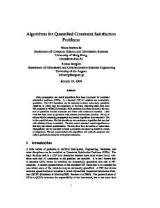
Fig. 2. Results for the Microgenetic Iterative Descent (mid)
40 35 30 25 20 15 10 5 0 0
0.24 0.25
10000 20000 30000 40000 50000 60000 70000 80000 90000 100000 evaluations 0.26 0.27
0.28 0.29
0.30 0.31
0.32 0.33
Fig. 1. Results for the co-evolutionary approach (ccs)
C.1 Effectiveness Looking at the effectiveness for low p values we can can distinguish four groups. The first group is formed by ccs, arc-ga and mid as they never find a solution, hence we do not include graphs for the sr (always zero) and the aes (always undefined). The second group contains the integer-based Standard ea, H-ga.2 and coe-h ga. These algorithms have similar performance. Their sr is between 2–4% on the easiest p = 0.24 degrading rather quickly for increasing values of p (implying unreliable aes values), but the mean error is showing only a rather moderate increase with p. The third group consists solely of the permutationbased Standard ea with a sr of almost 30%. Finally the fourth group consists of H-ga.1, H-ga.3, saw and the
Glass-Box algorithm. It is clearly distinguished by algorithms having a success rate larger than 80% at p = 0.24, which then degrade linearly with increasing p until almost zero at p = 0.30. When we compare the success rate graphs from algorithms in group four we find that the best performance is by H-ga.3, saw and Glass Box, where these algorithm are the best for a subset of p settings. The ce curves form bands of the same shape that show the convergence of the algorithm on the best found result. For all eas except saw these graphs show the same behaviour when the difficulty of the algorithm increases. The shapes of these graphs are similar for various p values, but they show worsening results for increasing p’s. At the same time we witness a linear incline of the average best number of violated constraints of the best individual at the end of a run. This tells us that the effort to find good partial instances becomes more difficult with equal steps over the increase of the parameter p. It should be noted that the ce and me curves for saw must be interpreted differently from those of the other eas. Because the weights wi are updated by adding the increment ∆w, the range of the fitness function values is continuously scaled up. This makes a direct comparison with other ce and me figures difficult. This effect is visible in the ten plots in Figure 9. Every 25 evaluations this vector is updated resulting in higher fitness function values if saw
TABLE XIII Ranking of the algorithms based on average number of evaluations to termination.
average mean error at termination (ME)
450
400
350
groups
algorithms
300
group 1 group 2
ccs, arc-ga, mid integer-based Standard ea, permutation-based Standard ea, H-ga.2, coe-h ga H-ga.1, saw H-ga.3, Glass-Box
250
group 3 group 4
200
150 0.24
0.26
0.28 0.3 p in Model E (csp difficulty)
0.32
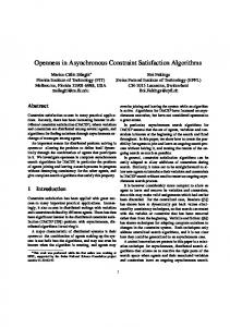
900
average champion error (CE)
800 700 600 500 400 300 200 100 0
10000 20000 30000 40000 50000 60000 70000 80000 90000 100000 evaluations
0.24 0.25
0.26 0.27
0.28 0.29
0.3 0.31
0.32 0.33
Fig. 3. Results for the arc-ga TABLE XII Ranking of algorithms based on success rate.
groups
algorithms
group group group group
ccs, arc-ga, mid integer-based Standard ea, H-ga.2, coe-h ga permutation-based Standard ea H-ga.1, H-ga.3, saw, Glass-Box
1 2 3 4
is not successful in resolving the uninstantiated variables of the best individual. We clearly see that for more difficult instances, i.e., higher values of p, the ce curves are steeper. The waving pattern in the plots is the result of the update process whereby the fitness values and thus the ce increases, after which it will decrease when the population is adapting to the new saw vector. In Table VII-C.1 we give a ranking of algorithms based on their success rates. The overall winner regarding success rates is the saw algorithm. C.2 Efficiency 1 Considering the number of fitness evaluations we can immediately distinguish the “looser group” containing the eas that never find a solution. These algorithms, mid, ccs, and arc-ga, always exhaust the maximum amount of 100,000
evaluations and the AES cannot be defined. Trying to compare the other eight algorithms by the aes values from Figures 1–11 it occurs that without further statistical analysis it is hard to establish if there are significant differences between their performances. Further inspection shows that for higher p’s with a corresponding low sr there are just a few data points to calculate the aes values, making the statistics unreliable. Therefore, statistical verification is carried out based on the average number of fitness evaluations to termination (aet). The difference with aes is that here all runs – and not only the successful ones – are taken into account. Using aet also makes the size of the resulting data sets in a comparison of two algorithms equal, regardless of their sr. We applied analysis of the variances (anova) and the t-test in the understanding that although the formal prerequisites of normal distribution and equal variance can not be guaranteed, these tests are robust in this respect. We performed anova with a confidence interval of 95% for each p from 0.24 to 0.33 and found that only for p = 0.31 were we unable to reject the null hypothesis of anova. This means that for all other p’s the results regarding aet are significantly different. However, for p = 0.32 and p = 0.33 the number of successful runs is very low causing borderline anova figures. Therefore, we decided to disregard results for p = 0.31, 0.32, 0.33 from further analysis. An ordering of the algorithms can be obtained by calculating two-sample t-tests of all combinations of the remaining eight eas. Because this is a multiple comparison procedure we have to use the Bonferroni Adjustment to adjust the significance level ([26], [41]). As the comparisons were made between eight algorithms, the resulting signifi= 0.05/28 = 0.0017857 with cance level is (1−0.95)/ 8·(8−1) 2 a confidence interval of 0.99821. We performed first a twosided two-sample t-test on all combinations of these eas followed by a single-sided two-sample t-test. This analysis indicates three groups, hence in total we can distinguish four groups again, as shown in Table XIII. The difference between these groups is significant with the Bonferroni adjustment. To identify an overall winner regarding efficiency measured by the number of fitness evaluations we find a secondary ordering among the best group showing a slight advantage of the Glass-Box ea.
TABLE XIV Number of conflict checks per evaluation for every evolutionary algorithm, ordered from small to large
Algorithm
Average
Standard deviation
Standard ea int. coe-h ga mid Standard ea perm. saw arc-ga H-ga.1 H-ga.2 Glass-Box H-ga.3 ccs
190.21 196.57 380.64 693.57 703.08 1270.8 1833.2 2089.8 2803.4 4707.8 20270
0.0279 5.7996 0.1505 38.407 21.119 16.780 24.075 0.2721 795.06 251.66 0.0000
C.3 Efficiency 2 Although fitness evaluations form a standard measure for comparing the efficiency of evolutionary algorithms, in some cases they do not show the whole truth. In our case the use of heuristics implies extra work that is invisible for this measure. To make this hidden work visible we measure the average number of conflict checks per evaluation, see Table XIV. This measure is calculated over all runs performed with each ea and gives a global indication of how much the aes and aet results are “cheating”. This measure shows large differences. We notice that poorly performing algorithms often use a low number of conflict checks per evaluation. Naturally, using more conflict checks gives opportunity to learn more about the problem instance at hand and be more successful in solving it. Looking at the top three heavy users of conflict checks we see two things. On the one hand, ccs is a particular case: it uses (an enormous amount of) conflict checks for fitness evaluation purposes, but not in heuristics. This explains why there is no correspondence between its (poor) performance and this measure. On the other hand, H-ga.3 and Glass-Box are among the best performing algorithms. It is remarkable that saw uses approximately 1/4 − th (vs. Glass-Box), respectively 1/7 − th (vs. H-ga.3) of conflict checks, but has better sr results than these algorithms. These observations relativate the ranking based on the number of fitness evaluations as given in the previous section. D. Comparison to classical methods This study would not be complete without comparing the performances of eas to traditional sound and complete constraint satisfaction algorithms. Earlier comparisons between classical methods and evolutionary algorithms on binary csps use the average number of conflict checks [34], [33] or the number of flips in [27]. Our comparison between classical and evolutionary algorithms is restricted to one very good traditional algorithm
and the best four eas from Table VII-C.1: H-ga.1, Hga.3, saw, Glass Box. To represent classical methods we choose forward checking with conflict-directed backjumping (fc-cbj), constructed using two techniques: forward checking, which originates from 1980 [30] and constraintdirected backjumping, which was added in 1993 [58]. As our test set only includes solvable instances and fc-cbj is a sound and complete algorithm, it always finds a solution and has a success rate of 1. Therefore, the results are only given by showing the average number of conflict checks, cf. Figure 12. Two important facts may be reported from this comparison. First that fc-cbj clearly outperforms the four evolutionary algorithms on both sr and on the average number of conflict checks. Second that for the test suite with respect to fc-cbj the most difficult instances lie at 0.31 and 0.32, which is a confirmation of the fact that we have performed our study in the mushy region. Another observation can be made in the comparisons of the four eas involved. Figure 12 shows that saw is faster than the other three algorithms on every setting of p, in terms of the number of constraint checks. VIII. Conclusions In this paper we have presented an overview of evolutionary algorithms that have been proposed to solve constraint satisfaction problems. We have compared these algorithms and a classical algorithm, forward checking with conflict-directed backjumping on the same test suite. This test suite has been created by a problem instance generator based on a recent theoretical model (model E). This generator and the instances are available on the Internet6 . Future studies of constraint satisfaction problem solvers can benefit from these, serving as benchmarks and thus making results comparable. Also the implemented algorithms are available on-line at http://www.cs.vu.nl/ ~bcraenen/JavaEa2. The outcomes of our experiments can be briefly summarised as follows: 1. The classical algorithm we used for benchmarking clearly wins from all evolutionary methods. 2. Certain eas that have been specifically tailored to csps — some heavily relying on heuristics — show no significant improvement over the Standard ea. The performance differences between these algorithms are small as if adding csp specific features would make no difference. 3. The best performing ea concerning effectivity (success rate) and efficiency (measured by the average number of conflict checks) is the saw algorithm. One possible reason for the second finding is that most heuristics in these algorithms are invented to exploit differences between constraints, i.e., concentrating the search on particularly difficult constraints, but the generated csp instances from model E have little inhomogeneity to exploit. 6 Generator: http://freshmeat.net/projects/randomcsp, instances: http://www.cs.vu.nl/~bcraenen/resources/csps_modelE_ v20_d20.tar.gz
In our opinion this does not invalidate the choice of the test suite or the generator, but indicates an interesting aspect. We believe that the hardness of many real world problems is caused by a cluster of hard to solve constraints within a larger network of easier ones. Algorithms with heuristics might be good at detecting this cluster — that might be relatively small — and solve the whole problem by solving this smaller problem well. Many studies — on finding where the real hard problems are — report this effect and “algorithm teasing” problem instance generators are often based on flattening out structures in order to withhold simple biases, for instance, on flat, equi-partite graphs for graph colouring [11]. From this perspective, our test suite can be seen as representing the very kernel of a hard problem and algorithms are compared on this kernel. The weakness of some heuristic based eas is counterbalanced by the fact that the best performing eas all involve heuristics too. Apparently, using heuristics can improve ea performance, but does not necessarily do so. Heuristics always introduce a bias enhancing exploitation, meanwhile reduce the exploration capabilities of the ea. It is therefore crucial to maintain a good balance between exploitation and exploration. The Glass-Box algorithm and saw form examples of the successful application of heuristics. They belong to the winning algorithms and outperform their respective benchmarks (integer-based standard ea and permutationbased standard ea, respectively), indicating that the applied heuristics are helpful. To reduce the possibly disadvantageous effects of heuristics, both algorithms include equally powerful explorational elements. Within saw the stepwise adaption of weights mechanism enables the algorithm to leave local optima and explore different parts of the search space. In the Glass-Box algorithm the classical elements of an ea, like crossover and mutation, make sure that enough exploration is done. A somewhat surprising variant of the heuristic eas is Hga.3 which combines the multi-parent heuristic crossover and the asexual heuristic operator replacing mutation. This setup sounds too much biased, but has one of the best performances of all algorithms, while the multi-parent heuristic crossover combined with random mutation (Hga.2) performs poorly. Apparently, applying the asexual heuristic operator after the multi-parent heuristic crossover forms a lucky combination, giving better results than combinations of these heuristic operators with random mutation. The application of heuristics, although improving ea performance measured in success rate and AES, comes at a price in terms of additional work hidden for measures based on the number of fitness evaluations. Table XIV shows that the Glass-Box ea and H-ga.3 use the most conflict checks per fitness evaluation (except for ccs). In this respect saw performs significantly better and among all eas it approaches the classical benchmark algorithm the closest, as the comparison in Figure 12 indicates. This comparative study gives suggestions for future research directions. Analysing the balance between the
heuristic bias and random exploration seems a promising subject. This might open the way to on-the-fly control of heuristics, which is especially interesting for it can reduce the amount of experimentation needed to calibrate heuristics correctly. References [1] [2] [3]
[4] [5] [6] [7]
[8]
[9]
[10]
[11]
[12] [13]
[14] [15]
[16]
D. Achlioptas, L.M. Kirousis, E. Kranakis, D. Krizanc, M.S.O. Molloy, and Y.C. Stamatiou. Random constraint satisfaction: A more accurate picture. Constraints, 4(6):329–344, 2001. Th. B¨ ack, editor. Proceedings of the 7th International Conference on Genetic Algorithms, San Francisco, CA, 1997. Morgan Kaufmann Publishers, Inc. Th. B¨ ack, A.E. Eiben, and M.E. Vink. A superior evolutionary algorithm for 3-SAT. In V.W. Porto, N. Saravanan, D. Waagen, and A.E. Eiben, editors, Proceedings of the 7th Annual Conference on Evolutionary Programming, number 1477 in Lecture Notes in Computer Science, pages 125–136, Berlin, 1998. Springer-Verlag. N. Barnier and P. Brisset. Optimization by hybridation of a genetic algorithm with constraint satisfaction techniques. In IEEE [40], pages 645–649. L. Booker. Improving search in genetic algorithms. In Genetic Algorithms and Simulated Annealing, pages 61–73. Morgan Kaufmann Publishers, Inc., 1987. J. Bowen and G. Dozier. Solving constraint satisfaction problems using a genetic/systematic search hybride that realizes when to quit. In Eshelman [25], pages 122–129. B.G.W. Craenen and A.E. Eiben. Stepwise adaption of weights with refinement and decay on constraint satisfaction problems. In L. Spector, E. Goodman, A. Wu, W.B. Langdon, H.-M. Voigt, M. Gen, S. Sen, M. Dorigo, S. Pezeshk, M. Garzon, and E. Burke, editors, Proceedings of the Genetic and Evolutionary Computation Conference, GECCO-2001, pages 291–298, San Francisco, CA, 2001. Morgan Kaufmann Publishers, Inc. B.G.W. Craenen, A.E. Eiben, and E. Marchiori. Solving constraint satisfaction problems with heuristic-based evolutionary algorithms. In Congress on Evolutionary Computation 2000. IEEE Computer Society Press, July 2000. B.G.W. Craenen, A.E. Eiben, and E. Marchiori. How to handle constraints with evolutionary algorithms. In L. Chambers, editor, The Practical Handbook of Genetic Algorithms: Applications, 2nd edition, volume 1, pages 341–361. Chapman & Hall/CRC, 2 edition, 2001. B.G.W. Craenen, A.E Eiben, E. Marchiori, and A. Steenbeek. Combining local search and fitness function adaptation in a GA for solving binary constraint satisfaction problems. In D. Whitley, D. Goldberg, E. Cant´ u-Paz, L. Spector, I. Parmee, , and H.G. Beyer, editors, Proceedings of the Genetic and Evolutionary Computation Conference (GECCO-2000), San Francisco, CA, 2000. Morgan Kaufmann Publishers, Inc. J.C. Culberson and F. Luo. Exploring the k-colorable landscape with iterated greedy. In M.A. Tricj and D.S. Johnson, editors, Second DIMACS Challenge, special issue, Series in Discrete Mathematics and Theoretical Computer Science. AMS, 1996. Available at http://web.cs.ualberta.ca/~joe/. G. Dozier, J. Bowen, and D. Bahler. Solving small and large constraint satisfaction problems using a heuristic-based microgenetic algorithm. In IEEE [37], pages 306–311. G. Dozier, J. Bowen, and D. Bahler. Solving randomly generated constraint satisfaction problems using a micro-evolutionary hybrid that evolves a population of hill-climbers. In Proceedings of the 2nd IEEE Conference on Evolutionary Computation, pages 614–619. IEEE Computer Society Press, 1995. G. Dozier, J. Bowen, and A. Homaifar. Solving constraint satisfaction problems using hybrid evolutionary search. Transactions on Evolutionary Computation, 2(1):23–33, 1998. A.E. Eiben. Evolutionary algorithms and constraint satisfaction: Definitions, survey, methodology, and research directions. In L. Kallel, B. Naudts, and A. Rogers, editors, Theoretical Aspects of Evolutionary Computating, Natural Computing, pages 13–58. Springer, 2001. A.E. Eiben, E.H.L. Aarts, K.M. van Hee, and W.P.M. Nuijten. A unifying view on heuristic search. Annals of Operations Research, 55:81–99, 1995.
[17] A.E. Eiben and J.K. van der Hauw. Adaptive penalties for evolutionary graph-coloring. In J.-K. Hao, E. Lutton, E. Ronald, M. Schoenauer, and D. Snyers, editors, Artificial Evolution ’97, number 1363 in Lecture Notes in Computer Science, pages 95– 106, Berlin, 1998. Springer-Verlag. [18] A.E. Eiben, J.K. van der Hauw, and J.I. van Hemert. Graph coloring with adaptive evolutionary algorithms. Journal of Heuristics, 4(1):25–46, 1998. [19] A.E. Eiben, J.I. van Hemert, E. Marchiori, and A.G. Steenbeek. Solving binary constraint satisfaction problems using evolutionary algorithms with an adaptive fitness function. In A.E. Eiben, Th. B¨ ack, M. Schoenauer, and H.-P. Schwefel, editors, Proceedings of the 5th Conference on Parallel Problem Solving from Nature, number 1498 in Lecture Notes in Computer Science, pages 196–205, Berlin, 1998. Springer-Verlag. [20] A.E. Eiben and J.I. van Hemert. SAW-ing EAs: Adapting the fitness function for solving constrained problems. In D. Corne, M. Dorigo, and F. Glover, editors, New Ideas in Optimization, pages 389–402. McGraw-Hill, 1999. [21] A.E. Eiben, P.-E. Rau´ e, and Zs. Ruttkay. Heuristic genetic algorithms for constrained problems, Part I: Principles. Technical Report IR-337, Vrije Universiteit Amsterdam, 1993. [22] A.E. Eiben, P-E. Rau´ e, and Zs. Ruttkay. Solving constraint satisfaction problems using genetic algorithms. In IEEE [37], pages 542–547. [23] A.E. Eiben, P.-E. Rau´ e, and Zs. Ruttkay. Constrained problems. In L. Chambers, editor, Practical Handbook of Genetic Algorithms, pages 307–365. CRC Press, 1995. [24] A.E. Eiben and Zs. Ruttkay. Self-adaptivity for constraint satisfaction: Learning penalty functions. In IEEE [38], pages 258– 261. [25] L.J. Eshelman, editor. Proceedings of the 6th International Conference on Genetic Algorithms. Morgan Kaufmann Publishers, Inc., 1995. [26] A. Feelders and W. Verkooijen. Which method learns the most data? methodological issues in the analysis of comparative studies. In Preliminary papers of the Fifth International Workshop on Artificial Intelligence and Statistics, pages 219–225, January 1995. [27] J. Gottlieb, E. Marchiori, and C. Rossi. Evolutionary algorithms for the satisfiability problem. Journal of Evolutionary Computation, 10(1):35–50, 2002. [28] H. Handa, N. Baba, O. Katai, T. Sawaragi, and T. Horiuchi. Genetic algorithm involving coevolution mechanism to search for effective genetic information. In IEEE [39]. [29] H. Handa, C. O. Katai, N. Baba, and T. Sawaragi. Solving constraint satisfaction problems by using coevolutionary genetic algorithms. In IEEE [40], pages 21–26. [30] R. Haralick and G. Elliot. Increasing tree search efficiency for constraint-satisfaction problems. Artificial Intelligence, 14(3rd):263–313, 1980. [31] J.K. van der Hauw. Evaluating and improving steady state evolutionary algorithms on constraint satisfaction problems. Master’s thesis, Leiden University, 1996. Also available as http: //www.liacs.nl/MScThesis/IR96-21.html. [32] J.I. van Hemert. Applying adaptive evolutionary algorithms to hard problems. Master’s thesis, Leiden University, 1998. Also available as http://www.liacs.nl/~jvhemert/publications/ IR-98-19.ps.gz. [33] J.I. van Hemert. Application of Evolutionary Computation to Constraint Satisfaction and Data Mining. PhD thesis, Leiden University, Leiden, The Netherlands, 2002. [34] J.I. van Hemert. Comparing classical methods for solving binary constraint satisfaction problems with state of the art evolutionary computation. In Stefano Cagnoni, Jens Gottlieb, Emma Hart, Martin Middendorf, and G¨ unther Raidl, editors, Applications of Evolutionary Computing, Proceedings of EvoWorkshops2002: EvoCOP, EvoIASP, EvoSTim, volume 2279 of lncs, pages 81–90, Kinsale, Ireland, 3-4 April 2002. SpringerVerlag. [35] J.I. van Hemert. Documentation for the RandomCsp library. Leiden University, 2002. Code and documentation at http://freshmeat.net/projects/randomcsp. [36] A. Hertz and D. Kobler. A framework for the description of evolutionary algorithms. European Journal of Operational Research, 126:1–12, 2000. [37] Proceedings of the 1st IEEE Conference on Evolutionary Computation. IEEE Computer Society Press, 1994.
[38] Proceedings of the 3rd IEEE Conference on Evolutionary Computation. IEEE Computer Society Press, 1996. [39] Proceedings of the 4th IEEE Conference on Evolutionary Computation. IEEE Computer Society Press, 1997. [40] Proceedings of the 5th IEEE Conference on Evolutionary Computation. IEEE Computer Society Press, 1998. [41] E.L. Korn and B.I. Graubard. Simultaneous testing of regression coefficients with complex survey data: use of bonferroni t statistics. The American Statistician, 44:270–276, 1990. [42] E. MacIntyre, P. Prosser, B.M. Smith, and T. Walsh. Random constraint satisfaction: theory meets practice. In M. Maher and J.-F. Puget, editors, Principles and Practice of Constraint Programming — CP98, pages 325–339, Berlin, 1998. SpringerVerlag. [43] E. Marchiori. Combining constraint processing and genetic algorithms for constraint satisfaction problems. In B¨ ack [2], pages 330–337. [44] E. Marchiori and A. Steenbeek. Genetic local search algorithm for random binary constraint satisfaction problems. In Proceedings of the ACM Symposium on Applied Computing, 2000. to appear. [45] Z. Michalewicz. Genetic algorithms, numerical optimization, and constraints. In Eshelman [25], pages 151–158. [46] Z. Michalewicz. A survey of constraint handling techniques in evolutionary computation methods. In J.R. McDonnell, R.G. Reynolds, and D.B. Fogel, editors, Proceedings of the 4th Annual Conference on Evolutionary Programming, pages 135–155, Cambridge, MA, 1995. MIT Press. [47] Z. Michalewicz and N. Attia. Evolutionary optimization of constrained problems. In A.V. Sebald and L.J. Fogel, editors, Proceedings of the 3rd Annual Conference on Evolutionary Programming, pages 98–108. World Scientific, 1994. [48] Z. Michalewicz, K. Deb, M. Schmidt, and T. Stidsen. Testcase generator for nonlinear continuous parameter optimization techniques. IEEE Transactions on Evolutionary Computation, 4(3):197–215, 2000. [49] Z. Michalewicz and M. Michalewicz. Pro-life versus prochoice strategies in evolutionary computation techniques. In M. Palaniswami, Y. Attikiouzel, R.J. Marks, D. Fogel, and T. Fukuda, editors, Computational Intelligence: A Dynamic System Perspective, pages 137–151. IEEE Computer Society Press, 1995. [50] Z. Michalewicz and M. Schmidt. TCG-2: A test-case generator for nonlinear parameter optimisation techniques. In A. Ghosh and S. Tsutsui, editors, Advances in Evolutionary Computating: Theory and Applications, pages 193–212. Springer, 2003. [51] Z. Michalewicz and M. Schoenauer. Evolutionary algorithms for constrained parameter optimization problems. Journal of Evolutionary Computation, 4(1):1–32, 1996. [52] P. Morris. The breakout method for escaping from local minima. In Proceedings of the 11th National Conference on Artificial Intelligence, AAAI-93, pages 40–45. AAAI Press/The MIT Press, 1993. [53] J. Paredis. Coevolutionary constraint satisfaction. In Y. Davidor, H.-P. Schwefel, and R. M¨ anner, editors, Proceedings of the 3rd Conference on Parallel Problem Solving from Nature, number 866 in Lecture Notes in Computer Science, pages 46–55, Berlin, 1994. Springer-Verlag. [54] J. Paredis. Co-evolutionary computation. Artificial Life, 2(4):355–375, 1995. [55] J. Paredis. Coevolving cellular automata: Be aware of the red queen. In B¨ ack [2]. [56] CSP problem instances using Model E http://www.cs.vu.nl/ ~bcraenen/resources/csps_modelE_v20_d20.tar.gz, 2002. [57] P. Prosser. An empirical study of phase transitions in binary constraint satisfaction problems. Journal of Artificial Intelligence, 81:81–109, 1996. [58] Patrick Prosser. Hybrid algorithms for the constraint satisfaction problem. Computational Intelligence, 9(3):268–299, August 1993. [59] J.T. Richardson, M.R. Palmer, G. Liepins, and M. Hilliard. Some guidelines for genetic algorithms with penalty functions. In Schaffer [65], pages 191–197. [60] M.C. Riff-Rojas. Using the knowledge of the constraint network to design an evolutionary algorithm that solves CSP. In IEEE [38], pages 279–284. [61] M.C. Riff-Rojas. Evolutionary search guided by the constraint network to solve CSP. In IEEE [39], pages 337–348.
0.1
success rate (SR)
0.08
0.06
0.04
0.02
0 0.24
0.26
0.28 0.3 p in Model E (csp difficulty)
0.32
average evaluations to a solution (AES)
100000
80000
60000
40000
20000
0 0.24
0.26
0.28 0.3 p in Model E (csp difficulty)
0.32
average mean error at termination (ME)
10
8
6
4
2
0 0.24
0.26
0.28
0.3
0.32
p in Model E (csp difficulty) 40 35 average champion error (CE)
[62] M.-C. Riff Rojas. A network-based adaptive evolutionary algorithm for constraint satisfaction problems. Meta-heuristics: Advances and Trends in Local Search Paradigms for Optimization, pages 325–339, 1998. [63] Francesca Rossi, Charles Petrie, and Vasant Dhar. On the equivalence of constraint satisfaction problems. In Luigia Carlucci Aiello, editor, ECAI’90: Proceedings of the 9th European Conference on Artificial Intelligence, pages 550–556, Stockholm, 1990. Pitman. [64] T. Runnarson and X. Yao. Constrained evolutionary optimization – the penalty function approach. In R. Sarker, M. Mohammadian, and X. Yao, editors, Evolutionary Optimization, chapter 4, pages 87–113. Kluwer Academic Publishers, 2002. [65] J.D. Schaffer, editor. Proceedings of the 3rd International Conference on Genetic Algorithms, San Mateo, California, 1989. Morgan Kaufmann Publishers, Inc. [66] M. Schoenauer and S. Xanthakis. Constrained GA optimization. In R.K. Belew and L.B. Booker, editors, Proceedings of the 4th International Conference on Genetic Algorithms, pages 573–580. Morgan Kaufmann Publishers, Inc., 1991. [67] B. Smith. In search of exceptionally difficult constraint satisfaction problems. Technical Report RR 94.2, University of Leeds, 1994. [68] B. Smith. The phase transition in constraint satisfaction problems: A closer look at the mushy region. Technical Report RR 93.41, University of Leeds, 1994. [69] B. Smith and S.A. Grant. Modelling exceptionally hard constraint satisfaction problems. In G. Smolka, editor, Principles and Practice of Constraint Programming — CP97, number 1330 in Lecture Notes in Computer Science, pages 182–195, Berlin, 1997. Springer-Verlag. [70] B.M. Smith. Phase transition and the mushy region in constraint satisfaction problems. In A.G. Cohn, editor, Proceedings of the 11th European Conference on Artificial Intelligence, pages 100– 104, New York, NY, 1994. John Wiley & Sons. [71] B.M. Smith and M.E. Dyer. Locating the phase transition in binary constraint satisfaction problems. Journal of Artificial Intelligence, 81(1-2):155–181, 1996. [72] Peter J. Stuckey and Vincent Tam. Improving evolutionary algorithms for efficient constraint satisfaction. International Journal on Artificial Intelligence Tools, 8(4):363–384, 1999. [73] P. van Hentenryck, V. Saraswat, and Y. Deville. Constraint processing in cc(FD). In A. Podelski, editor, Constraint Programming: Basics and Trends. Springer-Verlag, Berlin, 1995. [74] D. Whitley. The GENITOR algorithm and selection pressure: Why rank-based allocation of reproductive trials is best. In Schaffer [65], pages 116–123. [75] D. Whitley. Permutations. In T. B¨ ack, D.B. Fogel, and Z. Michalewicz, editors, Evolutionary Computation 1: Basic Algorithms and Operators, chapter 33.3, pages 274–284. Institute of Physics Publishing, 2000. [76] C.P. Williams and T. Hogg. Exploiting the deep structure of constraint problems. Journal of Artificial Intelligence, 70:73– 117, 1994.
30 25 20 15 10 5 0 0
0.24 0.25
10000 20000 30000 40000 50000 60000 70000 80000 90000 100000 evaluations 0.26 0.27
0.28 0.29
0.30 0.31
0.32 0.33
Fig. 4. Results for the Standard ea integer-based (note the scale of the y-axis of sr)
1
0.1
0.8
success rate (SR)
success rate (SR)
0.08
0.06
0.04
0 0.24
0.26
0.28 0.3 p in Model E (csp difficulty)
0 0.24
0.32
average evaluations to a solution (AES)
average evaluations to a solution (AES)
0.26
0.28 0.3 p in Model E (csp difficulty)
0.32
0.28 0.3 p in Model E (csp difficulty)
0.32
1100
100000
80000
60000
40000
20000
0 0.24
0.26
0.28 0.3 p in Model E (csp difficulty)
1000 900 800 700 600 500 400 300 0.24
0.32
0.26
10
average mean error at termination (ME)
10
average mean error at termination (ME)
0.4
0.2
0.02
8
6
4
2
0 0.24
0.26
0.28 0.3 p in Model E (csp difficulty)
8
6
4
2
0 0.24
0.32
0.26
0.28
0.3
0.32
p in Model E (csp difficulty) 4.5
40
4 average champion error (CE)
35 average champion error (CE)
0.6
30 25 20 15 10
3.5 3 2.5 2 1.5
5 1
0 0
0.24 0.25
0
10000 20000 30000 40000 50000 60000 70000 80000 90000 100000 evaluations 0.26 0.27
0.28 0.29
0.3 0.31
0.32 0.33
Fig. 5. Results for the H-ga.2 (note the scale of the y-axis of sr)
0.24 0.25
20000
0.26 0.27
40000 60000 evaluations 0.28 0.29
0.3 0.31
80000
100000
0.32 0.33
Fig. 6. Results for the Standard EA permutation-based (note the scale of the y-axis of aes and ce)
1
0.08
0.8
success rate (SR)
success rate (SR)
0.1
0.06
0.04
0.02
0.26
0.28 0.3 p in Model E (csp difficulty)
0 0.24
0.32
80000
60000
40000
20000
0 0.24
0.26
0.28 0.3 p in Model E (csp difficulty)
0.28 0.3 p in Model E (csp difficulty)
0.32
80000
60000
40000
20000
0 0.24
0.32
0.26
0.28
0.3
0.32
p in Model E (csp difficulty)
10
average mean error at termination (ME)
10
8
6
4
2
0 0.24
0.26
0.28 0.3 p in Model E (csp difficulty)
8
6
4
2
0 0.24
0.32
40
35
35 average champion error (CE)
40
30 25 20 15 10 5
0.26
0.28 0.3 p in Model E (csp difficulty)
0.32
30 25 20 15 10 5
0
0 0
0.24 0.25
0.26
100000
average evaluations to a solution (AES)
average evaluations to a solution (AES)
100000
average mean error at termination (ME)
0.4
0.2
0 0.24
average champion error (CE)
0.6
10000 20000 30000 40000 50000 60000 70000 80000 90000 100000 evaluations 0.26 0.27
0.28 0.29
0.30 0.31
0.32 0.33
Fig. 7. Results for the coe-h ga (note the scale of the y-axis of sr)
0
0.24 0.25
20000
0.26 0.27
40000 60000 evaluations 0.28 0.29
0.3 0.31
80000
0.32 0.33
Fig. 8. Results for the Glass-Box ga
100000
1
1
0.8
success rate (SR)
success rate (SR)
0.8
0.6
0.4
0.2
0.4
0.2
0 0.24
0.26
0.28 0.3 p in Model E (csp difficulty)
0 0.24
0.32
100000
0.26
0.28 0.3 p in Model E (csp difficulty)
0.32
100000
average evaluations to a solution (AES)
average evaluations to a solution (AES)
0.6
80000
60000
40000
20000
0 0.24
0.26
0.28 0.3 p in Model E (csp difficulty)
80000
60000
40000
20000
0 0.24
0.32
0.26
0.28
0.3
0.32
p in Model E (csp difficulty)
200
10
average mean error at termination (ME)
average mean error at termination (ME)
180 160 140 120 100 80 60 40 20 0 0.24
0.26
0.28
0.3
8
6
4
2
0 0.24
0.32
p in Model E (csp difficulty) 200
0.26
0.28 0.3 p in Model E (csp difficulty)
0.32
40 35
160 average champion error (CE)
average champion error (CE)
180
140 120 100 80 60 40 20
25 20 15 10 5
0 0
0.24 0.25
30
10000 20000 30000 40000 50000 60000 70000 80000 90000 100000 evaluations 0.26 0.27
0.28 0.29
0.3 0.31
0.32 0.33
Fig. 9. Results for the Stepwise Adaptation of Weights ea (saw) (note the scale of the y-axis of me and ce)
0 0
0.24 0.25
10000 20000 30000 40000 50000 60000 70000 80000 90000 100000 evaluations 0.26 0.27
0.28 0.29
0.3 0.31
Fig. 10. Results for the H-ga.1
0.32 0.33
1
success rate (SR)
0.8
0.6
0.4
0.2
0 0.24
0.26
0.28 0.3 p in Model E (csp difficulty)
0.32
80000
60000
5e+08 4.5e+08
40000
4e+08 20000
0 0.24
0.26
0.28
0.3
0.32
p in Model E (csp difficulty)
average mean error at termination (ME)
10
H.GA-1 H.GA-3 Glass Box SAW FC-CBJ
3.5e+08 3e+08 2.5e+08 2e+08 1.5e+08 1e+08
8
5e+07 0 0.24
6
0.26
0.28
0.3
0.32
p in Model E (csp difficulty) 4
Fig. 12. Comparing the evolutionary algorithms H-ga.1, H-ga.3, Glass-Box and saw with the complete approach fc-cbj on the average number of conflict checks performed during a run
2
0 0.24
0.26
0.28 0.3 p in Model E (csp difficulty)
0.32
40 35 average champion error (CE)
average conflict checks
average evaluations to a solution (AES)
100000
30 25 20 15 10 5 0 0
0.24 0.25
10000 20000 30000 40000 50000 60000 70000 80000 90000 100000 evaluations 0.26 0.27
0.28 0.29
0.3 0.31
Fig. 11. Results for the H-ga.3
0.32 0.33