Electronic Notes in Theoretical Computer Science 62 (2002) URL: http://www.elsevier.nl/locate/entcs/volume62.html 21 pages
Comparing Higher-Order Encodings in Logical Frameworks and Tile Logic 1 Roberto Bruni, a Furio Honsell, b Marina Lenisa, b and Marino Miculan b a
Dipartimento di Informatica, Universit` a di Pisa Corso Italia 40, 56125 Pisa, Italy.
[email protected] b
Dipartimento di Matematica e Informatica, Universit` a di Udine Via delle Scienze 206, 33100 Udine, Italy. honsell,lenisa,
[email protected]
Abstract In recent years, logical frameworks and tile logic have been separately proposed by our research groups, respectively in Udine and in Pisa, as suitable metalanguages with higher-order features for encoding and studying nominal calculi. This paper discusses the main features of the two approaches, tracing differences and analogies on the basis of two case studies: late π-calculus and lazy simply typed λ-calculus.
Introduction A key area of research of the tosca project was concerned with the topic of metalanguages and (computational) metamodels, and in particular with their use as logic and semantic frameworks for the definition and analysis of languages, calculi and programming paradigms. A metalanguage can be seen as a general specification system which allows for representing, in a uniform setting, a wide range of formal systems, referred to as the object systems. More precisely, a metalanguage is composed by two parts: a formal language, the formalism, and an informal encoding methodology, or protocol, which describes how an object system can be represented in the formalism guaranteeing suitable properties. The metalanguage has to be expressive enough to allow for a faithful translation, the specification, of all components of the object systems. Peculiarites and idiosincrasies of the object systems must be taken into account, e.g. context-dependent features such as binders, non-standard notions of substitution, fresh name creation, weird side conditions, etc. Still, the formalism must strive for simplicity and it should be implementable on a machine. Indeed, such a general-purpose implementation 1
Research supported by the MURST Project tosca.
c °2002 Published by Elsevier Science B. V.
Bruni et al.
can be readily turned into a mechanized proof assistant for any given object system, by simply providing the specification. This is particularly useful in the case of logics and formal systems for dealing with programs and processes properties. We can factorize out most of the common features of the plethora of program and process logics, thus avoiding the daunting task of implementing a specific proof assistant or integrated environment for each of them. Three research groups of the tosca project, in Milano, Pisa and Udine, have been actively involved in the area of metalanguages and metamodels developing and experimenting cospan-span categories, tile logic (tl) [14, 4] and logical frameworks (e.g. lf) [15, 27], respectively. We refer the reader to [13] for a comparison between the two first metamodels. In this paper, we discuss tile logic and logical frameworks. The foundations of both metamodels are by now well established, various tools based on them are available (e.g. [19, 7]), and several case studies concerning widely used calculi and programming paradigms have been carried out. The two approaches have been developed separately and have focused on different aspects and problems of meta-representation, namely syntactic and proof-theoretical for the Logical Frameworks, and semantical and categorical for tile logic. The two approaches however share many features both from the conceptual and the methodological viewpoint. Thus, in the spirit of the tosca project, it is interesting to clarify these connections, allowing for bidirectional technology transfer, inheritance and reuse of techniques. In this paper we address this issue and try to shed some light on the analogies (but also on the differences) between the two approaches by comparing the encodings in tl and lf of two paradigmatic nominal calculi: λ-calculus and πcalculus. A key technique for their translations in lf and tl is the possibility of exploiting higher-order objects as first-class citizens, so to delegate namehandling issues (name binding, capture avoiding substitution, α-conversion, name hiding, fresh name creation) to the underlying machinery, where these are dealt with automatically, in a standard way. We remark that the choice of the two case studies is instrumental in comparing tl and lf, and not in claiming the novelty of the encoding themselves. In lf this encoding protocol is named Higher-Order Abstract Syntax (HOAS), while in tl the analogous idea leads to Higher-Order Tile Logic (HOTL). A main difference between the two approaches is that in HOAS the syntax plays a primary rˆole, while HOTL is strongly typed and provides the encoding with observational and operational semantics, and with categorical model of proof terms, i.e., HOTL could be called Higher-Order Abstract Semantics. Synopsys. In Section 1 we present the two metalanguages we focus on, namely the Edinburgh Logical Framework (lf) and the Tile Logic (tl). Sections 2 and 3 present the π-calculus and λ-calculus case studies, respectively. For each of them, we briefly present the object system, the formalization both in lf and tl, and we discuss and compare these encoding. Final remarks and directions for future work are in Section 4. 2
Bruni et al.
1
The two Metalanguages and Encoding Protocols
1.1 Logical Frameworks based on Type Theory Type Theories, such as the Edinburgh Logical Framework lf [15, 2] or the Calculus of (Co)Inductive Constructions [19] were especially designed, or can be fruitfully used, as a general logic specification language, i.e. as a Logical Framework (LF). In an LF, we can represent faithfully and uniformly all the relevant concepts of the inferential process in a logical system (syntactic categories, terms, variables, contexts, assertions, axiom schemata, rule schemata, instantiation, tactics, etc.) via the “judgements-as-types, λ-terms-as-proofs” paradigm. The key concept for representing assertions and rules is that of Martin-L¨of’s hypothetico-general judgement [22], which is rendered as a type of the dependent typed λ-calculus of the Logical Framework. The λ-calculus metalanguage of an LF supports Higher-Order Abstract Syntax (HOAS) `a la Church, i.e., syntax where language constructors may have higher order types. In HOAS, metalanguage variables play the rˆole of “object logic” variables so that schemata are represented as λ-abstractions and object-level instantiation amounts to metalanguage β-reduction. Hence, binding operators of the object language are encoded as higher order constants, being viewed as ranging over schemata. Thus, most of the machinery needed for handling names, such as capture-avoiding substitution, α-conversion of bound variables, generation of fresh names and instantiation of schemata, comes “for free” because it is safely delegated to the metalanguage [28]. Since LF’s allow for higher order assertions one can treat on a par axioms and rules, theorems and derived rules, and hence encode also generalized natural deduction systems in the sense of [31]. The LF specification of a formal system is given by a signature, i.e. a declaration of typed constants according to the following methodology: Theory of Syntax Syntactic categories of the object language are encoded as type constants; each syntactic constructor is encoded as a term constant of the appropriate type. Theory of Proofs Judgements over the object language are encoded as constants of “typed-valued function” kind, and each rule is encoded as a term constant of the appropriate type. Hence, derivations of a given assertion are represented as terms of the type corresponding to the assertion in question, so that checking the correctness of a derivation amounts just to type-checking in the metalanguage. Thus, derivability of an assertion corresponds to the inhabitation of the type corresponding to that assertion, i.e. the existence of a term of that type. It is possible to prove, informally but rigorously, that a formal system is adequately, faithfully represented by its encoding. This proof usually exhibit bijective maps between objects of the formal system (terms, formulæ, proofs) and the λ-terms (in canonical form) of the corresponding types in the formalization. 3
Bruni et al.
Encodings in LF’s often provide the “normative” formalization of the system under consideration. The specification methodology of LF’s, in fact, forces the user to make precise all tacit, or informal, conventions, which always accompany any presentation of a system. Any interactive proof development environment for the type theoretic metalanguage of an LF (e.g. Coq [19], LEGO [29]), can be readily turned into one for a specific logic, once we have defined the corresponding signature. Such a generated editor allows the user to reason “under assumptions” and go about in developing a proof the way mathematicians normally reason: using hypotheses, formulating conjectures, storing and retrieving lemmata, often in top-down, goal-directed fashion. In this paper we will adopt the Edinburgh Logical Framework lf [15]. lf is a system for deriving typing assertions of the shape Γ ` P : Q, whose intended meaning is “in the environment Γ, P is classified by Q”. Three kinds of entities are involved, i.e. terms (ranged over by M, N ), types and typed valued functions (ranged over by A, B), and kinds (ranged over by K). Types are used to classify terms, and kinds are used to classify types and typed valued functions. These entities are defined by the following abstract syntax. Π is the dependent type constructor. Intuitively Πx:A .B(x) denotes M ::= x | M N | λx : A.M the type of those functions, f , whose A ::= X | AM | Πx:A .B | λx : A.B domain is A and whose values belong to a codomain depending on the inK ::= Type | Πx:A .K. put, i.e. f (a) ∈ B(a), for all a ∈ A. Hence, A → B is just notation abbreviating Πx:A .B, when x does not occur free in B (x 6∈ F V (B)). In the “judgements-as-types” analogy the dependent product type Πx:A .B(x) represents the assertion “for all x ∈ A, B(x) holds”. Environments (ranged over by Γ, ∆) are lists of typed variables. A signature Σ is a particular environment which represents an object logic. Due to this different rˆole of signatures, instead of Σ, Γ ` P : Q we will write Γ `Σ P : Q; possibly we will drop the index Σ when clear from the context. We will say that a type A is inhabited in the environment Γ (and signature Σ) (denoted Γ `Σ : A) if there exists a term M such that Γ `Σ M : A. 1.2 Tile Logic Tile logic is a sequent calculus over a rule-based model (tile model ) whose sequents, called tiles, have a bidimensional nature: the horizontal dimension is devoted to the static structure of system configurations, while the vertical dimension is devoted to the observational dynamics of the system. Moreover, the operational rules are designed for open configurations, which may interact through their interfaces. In fact, unlike rewriting logic (rl) [23], where rewrite rules can be freely instantiated and contextualized (e.g., if f (x) ⇒ g(x) is a rule, then C[f (t)] can be rewritten to C[g(t)] for any context C[·] and any 4
Bruni et al.
initial configuration
initial input interface (i .i .i ) ³º´¹¸µ¶· trigger
º³/ ´¹µ¸·¶ initial output interface (i .o.i )
s
a
final input interface (f .i .i .)
b
³º´¹¸²µ¶·
º/³´¹µ¸² ·
t
effect
final output interface (f .o.i .)
final configuration
Fig. 1. A tile.
term t), tiles have the form in Figure 1 (whence the name), written as the a sequent s −→ t, stating that the initial configuration s evolves to the final b configuration t producing the effect b, but such a step is allowed only if the subcomponents of s evolve to the subcomponents of t, producing the trigger a a (e.g., the tile f (x) −→ g(x) can be applied to C[f (t)] only if t evolves with b effect a and a move of C[·] exists that is triggered by b). Triggers and effects are called observations and tile vertices are called interfaces. Formally, a tile system is a tuple R = (H, V, N, R) where H and V are monoidal categories with the same set of objects OH = OV , N is the set of rule names and R : N → AH × AV × AV × AH associates each name in x ∈ N a with a tile R(x) : s −→ t, with s, t ∈ H and a, b ∈ V. b
Tiles can be composed horizontally ( ∗ ), synchronizing an effect with a trigger; vertically ( · ), extending computations of a component; and in parallel ( ⊗ ), modeling concurrent steps. We say that a tile α is entailed by R, written R ` α, if α can be obtained by composing basic and auxiliary tiles via ∗, · and ⊗. These compositions satisfy the laws of monoidal double a b categories [14, 24]. For α : s −→ idx and β : t −→ idy with x the i.i.i. of β, idx
idy
id
t
x we write α / β as a shorthand for (α ∗ 1 ) · β. Similarly, for α : idx −→ s
a
idy
s
and β : idy −→ t with y the f.o.i. of α, we write α . β for α · (1 ∗ β). These b compositions are called diagonal and yield two monoidal categories. Though the direction of the arrows in Figure 1 follows the intuitive way of composing states (from left to right) and computations (from top to down), opposites categories can be as well considered, as done e.g. in [10, 11], when this is convenient to model certain operational features, and this impacts in reversing the direction of arrows either in one dimension or in both. tl extends the ordinary observational equivalences such as trace semantics and bisimilarity by taking htrigger, effecti pairs as labels, favoring the application of coalgebraic techniques to open systems [12]. The resulting abstract semantics are called tile trace equivalence and tile bisimilarity (these are families of equivalences indexed by sources and targets of configurations). It is often convenient to consider tile logics whose categories of configurations and observations are freely generated by suitable signatures ΣH and ΣV . In particular, when the categories of configurations and observations rely on 5
Bruni et al.
the same algebraic structure (e.g. symmetric monoidal, or cartesian), some auxiliary tiles can be added for free, which guarantee the consistency between the adjoined structure (e.g., symmetries or cartesianity), and the categorical models for such systems must be taken in the corresponding categories of, e.g., symmetric monoidal double categories or cartesian double categories [9, 4]. Fixing the auxiliary tiles and the format of the basic tiles of the system means fixing a tile format. Several (first order) tile formats have been e.g. defined which guarantee that tile bisimilarity is a congruence [5] (they usually exploit the format independent tile decomposition property [14] to prove the result). Though at present no automated verification tool is available which is based directly on tl, some prototyping has been made possible for suitable tl specification classes, via a conservative encoding in rl, as reported in [7, 8, 6]. The methodology of application of tl can be divided in three steps, which can mutually influence each other’s design decisions: Theory of Configurations Fix the signature of configurations identifying the syntactic constructors and freely adjoin the auxiliary structure needed in the category of configurations; Theory of Observations Fix the signature of observations (e.g. ordinary lts’s labels are usually seen as unary operators) and freely adjoin the auxiliary structure needed in the category of observations; Theory of Tiles Define the basic operational rules for the dynamics of system components, and fix the auxiliary tiles to be freely adjoined. In this paper we focus on the higher-order version of tiles introduced in [10], where H and V are cartesian closed, the models are cartesian closed double categories (ccdc), and the auxiliary tiles can be conveniently represented as those in the quartet category 2 of the cartesian closed category freely generated by the signature with the same sorts as ΣH and ΣV but empty set of operators. Due to space limitation, we refer to [10] for more details, giving here just the basic syntax and features of HOTL. The first thing to notice is that language constructors can have higher-order types and that λ-abstraction and application are introduced automatically in H and V. At the level of tiles instead we deal with object abstraction only (configuration and observation abstractions are in fact contra-variant and cannot be correctly typed in the ccdc framework). However, we can pass an argument (e.g. names in nominal calculi) which is bound in the initial configuration to the effect, providing bidimensional scope rules. The possibility of reconciling horizontal abstraction with vertical application is another interesting feature, proper of ccdc’s. Higher-order tiles are presented by typed sentences in the double λ-notation of [10]. To deal with the double λ-notation, type judgments Γ ` M : σ, where Γ is an environment and σ is the type of the term M in Γ, must take into account that terms are double cells and that their types, called contour types, 2
The quartet category of a category C is the double category of commuting squares in C.
6
Bruni et al.
are cell borders. Thus, a double signature is a 4-tuple Σ = hB, H, V, C i, where B is the set of type constants, H is the set of horizontal term constants h : σ, g : τ, . . . typed over B (note that σ, τ can also be higher-order types), V is the set of vertical term constants v : σ, u : τ, . . . typed over B, and C is the set of tile term constants α2s, β 2t, . . . , with s, t, . . . closed contour types. V :ρ A generic contour type has the form H : τ U :τ →σ / G : ρ → σ , where H and G are horizontal terms, while U and V are vertical terms. A contour type is well-typed under Γ if H, G, V and U are well-typed under Γ. A contour type is closed if it can be typed by an empty environment, i.e., if H, G, V and U are closed terms. Starting from the constants in Σ, more complex terms are constructed according to the syntax: M ::= α | h | v | x | ? | hM, M i% | Proj %i M | λ% x : σ.M | M @% M | M %M where α ∈ C, h ∈ H, v ∈ V, x is a generic variable, ? is the unit, and pairings, projections, abstractions and applications (the latter denoted by @) are feasible in all compositional dimensions of tiles as % ∈ {∗, ·, /, .} (horizontal, vertical and diagonal, the latter in the two distinct ways previously defined). Moreover, horizontal, vertical and diagonal compositions are also given, because abstraction is restricted to objects, and hence these compositions cannot be expressed just by functional application. A generic type sentence for double V :ρ λ-terms has the form Γ ` M 2 H : τ U :τ →σ / G : ρ → σ . We refer to [10] for the description of the type system, but it is worth remarking that all variables in Γ are propagated by default around the contour of the tiles, so that names in Γ can be used in U and G without being explicitly forwarded by H and V , this makes Γ be a global environment for typing M and its contour type. When a name x in Γ is abstracted from M , then the abstraction consistently binds the occurrences of x in H, V , U and G.
2
π-calculus with Late Semantics
2.1 The object system In this section we give the syntax of a finitary but significant fragment of the π-calculus, the late operational semantics, and the strong late bisimilarity equivalence, see [26] for more details. Let N be an infinite set of names, ranged over by x, y. The set of processes (or agents) P, ranged over by P , Q, is defined by the following abstract syntax: P ::= 0 | x¯y.P | x(y).P | τ.P | (νx)P | P1 |P2 | [x = y]P The input prefix operator x(y) and the restriction operator (νy) bind the occurrences of y in the argument P . Thus, for each process P we can define the sets of its free names fn(P ), bound names bn(P ) and names n(P ). Agents are 7
Bruni et al.
−
w 6∈ fn((νz)P )
x(w)
(IN)
x(z).P −→ P {w/z} µ
P0
P −→ µ
P |Q −→ P 0 |Q x(w)
P −→
Q −→
P −→ µ
(νy)P −→ (νy)P 0
x(z)
xy
P −→ P 0 Q −→ Q0 τ
(CLOSEl )
P |Q −→ (νw)(P 0 |Q0 ) P0
(PARl )
P |Q −→ P 0 {y/z}|Q0
Q0
τ
µ
(OUT)
xy
xy.P −→ P
bn(µ) ∩ fn(Q) = ∅
x(w)
P0
−
µ
P −→ P 0 µ
y 6∈ n(µ)inP isaandU dine (RES)
(COMl )
[x = x]P −→ P 0 − τ
τ.P −→ P
(MATCH) (TAU)
xy
P −→ P 0 x(w)
(νy)P −→
y 6= x, w 6∈ fn((νy)P 0 )
(OPEN)
P 0 {w/y}
Fig. 2. Late operational semantics of π-calculus.
taken up-to α-equivalence. For X ⊂ N , we let PX , {P ∈ P | fn(P ) ⊆ X}. Capture-avoiding substitution of y in place of x in P is denoted by P {y/x}. There is a plethora of slightly different lts’s for the late operational semantics of π-calculus, e.g. [26, 25, 30]. We present the original one in [26]: the µ relation −→ is the smallest relation on processes, satisfying the rules in Figure 2 (with the obvious rules PARr and COMr omitted). There are four kinds of actions, ranged over by µ. Action τ is the silent move, and x¯y is the free x ¯y output: P −→ Q means that P can reduce itself to Q emitting y on the chanx(z)
nel x. Dually, the input P −→ Q means that P can receive from the channel x(z)
x any name w and then evolve into Q{w/z}. The bound output P −→ Q means that P can evolve into Q emitting on the channel x a restricted name z of P (name extrusion). The channel x is called the subject, while z, y are the objects. The τ and free output are free actions, the other two are said bound. The functions fn(·), n(·) and bn(·) are extended to actions in the obvious way. Definition 2.1 A relation S ⊆ P × P is a strong late simulation iff, for all processes P, Q, if P S Q then µ
µ
(i) if P −→ P 0 and µ is free, then for some Q0 , Q −→ Q0 and P 0 S Q0 ; x(y)
x(y)
(ii) if P −→ P 0 and y 6∈ fn(P, Q), then for some Q0 , Q −→ Q0 and for all w ∈ N : P 0 {w/y} S Q0 {w/y}; x(y)
x(y)
(iii) if P −→ P 0 and y 6∈ fn(P, Q), then for some Q0 , Q −→ Q0 and P 0 S Q0 . S is a strong late bisimulation if both S and S −1 are strong late simulations. P . and Q are strong late bisimilar, 3 written P ∼ Q, if a strong late bisimulation .
3
It is well-known that strong late bisimilarity ∼ can be defined as the greatest fixed point of a suitable monotonic operator over subsets of P × P.
8
Bruni et al.
S exists such that P S Q. 2.2 Encoding the π-calculus in Logical Framework In this section we present an encoding of π-calculus in lf, which follows [16], further elaborated in [18] in the Calculus of Inductive Constructions. The corresponding lf signature Σπ appears in Figure 3. Syntax. Following the methodology outlined in Section 1.1, for each syntactic category of names, labels and processes we introduce a specific type. Syntactic constructors are defined for labels and processes only: names have no constructor, so that the only terms which can inhabit Name are metalevel variables, as usual in weak HOAS encodings [18, 17]. Binders of π-calculus are rendered in lf making use of suitable abstractions. In the case of the input prefix, for instance, in order to obtain a process, both a name (the input channel) and an abstraction (a function from names to processes) are required. Given a finite set of names X, it is easy to define an encoding function εX from π-calculus processes with free names in X, to lf terms of type Proc. Most of the π-calculus constructors are translated in the obvious way, but for input prefix εX (x(y).P ) = inp (x, λy : Name.εX∪{y} (P )) and restrictions: εX ((νy)P ) = ν(λy : Name.εX∪{y} (P )). Accordingly, π-calculus processes will be often pretty-printed, following the notation of Section 2.1. This encoding map is an adequate and faithful representation of the syntax of π-calculus: Proposition 2.2 (Adequacy, I) Let X = {x1 , . . . , xn } be a finite set of names. The map εX is a bijection between PX and the normal forms of type Proc in the signature Σπ and environment ΓX , {x1 : Name, . . . , xn : Name}. We omit the proof which follows a standard argument by induction on the syntax of terms and on the derivation of the typing judgement [15]. In view of the remarks above, the set fn(P ) for P ∈ Proc is simply the set of free variables of type Name, occurring in the canonical (normal) form of P . Operational semantics. The transition relation is rendered by two mutually defined inductive predicates 7−→, 7−→, → which take care of transitions involving free actions and bound actions, respectively. In the latter case, the result of the transition is not a process but a process context, i.e. a process with a hole, conveniently represented by a function Name → Proc. Rules for 7−→ and 7−→ → appear in Figure 3. Some of the rules of Figure 2 have two counterparts, according to whether they refer to free or bound transitions; the bound version of COND has been omitted together with the right versions of PAR, COM and CLOSE. Note that bound names in bound actions (the objects of communication) disappear in the encoding. In fact, the rˆole played by the objects in bound actions is to denote which name in the resulting process is bound by the action. Since these bound names in processes are denoted by “holes” in the encoding, taking full advantage of the HOAS approach, 9
Bruni et al.
Syntactic categories and constructors Name : Type 0 : Proc Label : Type τp : Proc → Proc Proc : Type inp : Name → (Name → Proc) → Proc τ : Label outp : Name → Name → Proc → Proc out : Name → Name → Label | : Proc → Proc → Proc in : Name → Label ν : (Name → Proc) → Proc bout : Name → Label [ = ] : Name → Name → Proc → Proc Judgements and rules 7−→ : Proc → Label → Proc → Type 7−→ → : Proc → Label → (Name → Proc) → Type τ
T AU : ΠP :Proc .τp .P 7−→ P out(x,y)
OU T : ΠP :Proc Πx,y:Name .outp (x, y).P 7−→ P in(x)
IN : ΠP :Name→Proc Πx:Name .inp (x).P 7−→ →P µ
µ
P ARlf : ΠP,Q,R:Proc Πµ:Label .P 7−→ R → (P |Q) 7−→ (R|Q) P ARlb : ΠP,Q:Proc ΠR:Name→Proc Πµ:Name→Label . µ
µ
P 7−→ → R → (P |Q) 7−→ → λx : Name. (Rx)|Q COMl : ΠP,Q,R:Proc ΠS:Name→Proc . out(x,y)
in(x)
τ
Πx,y:Name .P 7−→ R → Q 7−→ → S → (P |Q) 7−→ R|(Sy) ³ ´ µ µ RES f : ΠP,Q:Name→Proc Πµ:Label . Πx:Name .(P x) 7−→ (Qx) → ν(P ) 7−→ ν(Q) RES b : ΠP :Name→Proc ΠQ:Name→Name→Proc Πµ:Label . ³ ´ µ µ Πx:Name .(P x) 7−→ → (Qx) → ν(P ) 7−→ → λz : Name. ν(λx : Name.(Qxz)) µ ¶ in(x) bout(x) OP EN : ΠP,Q:Name→Proc Πx:Name . Πy:Name .(P y) 7−→ (Qy) → ν(P ) 7−→ → Q CLOSEl : ΠP,Q:Proc ΠR,S:Name→Proc Πx:Name . in(x)
bout(x)
τ
P 7−→ → R → Q 7−→ → S → (P |Q) 7−→ ν(λz : Name.(Rz)|(Sz)) µ
µ
CON Df : ΠP,Q:Proc Πµ:Label Πx:Name .P 7−→ Q → [x=x]P 7−→ Q Fig. 3. Σπ , lf signature for the π-calculus.
their representation in the bound action is unnecessary, e.g., the transition x(y)
in(x)
x(y).P 7−→ P is represented by in(x)(λy : Name.ε(P )) 7−→ → λy : Name.ε(P ). As an example, consider rule IN , where the target process is an abstraction; when an input occurs (e.g., in the COMl rule), the target is applied to the effectively received name, so that this name replaces all the occurrences of the placeholder in the target process. 10
Bruni et al.
The operational semantics we have presented here allows to eliminate those explicit side-conditions, which are needed in the ordinary semantics to enforce bound names to be fresh, so as to avoid name clashing. The side conditions are implicit in the higher-order nature of the type encoding of the rules in the lf presentation. Bound names remain bound also when the transition is performed, since abstractions are used for the target process. It is possible to establish a precise correspondence between derivations of the semantics of π-calculus and lf judgements derivable in the signature Σπ . Proposition 2.3 (Adequacy II) For any X ⊂fin N , P, Q ∈ PX , x, y ∈ N : τ
τ
: εX (P ) 7−→ εX (Q);
x ¯y
: εX (P ) 7−→ εX (Q);
•
P −→ Q iff ΓX `Σπ
•
P −→ Q iff ΓX `Σπ
•
P −→ Q iff ΓX `Σπ
•
P −→ Q iff ΓX `Σπ
x(y) x ¯(y)
out(x,y) in(x)
: εX (P ) 7−→ → λy : Name.εX∪{y} (Q); bout(x)
: εX (P ) 7−→ → λy : Name.εX∪{y} (Q).
The proof of this proposition is by induction on the structure of derivations (⇒) and on the structure of normal forms (⇐). The proposition above is proof-irrelevant, that is we do not consider the “proofs” corrisponding to the derivations of the transitions. This result can be strenghtened by considering also the structure of derivations of the lts, instead of the mere transitions. From this proof-theoretical point of view, there is a τ compositional bijection between derivations of P −→ Q and canonical forms τ t such that ΓX `Σπ t : εX (P ) 7−→ εX (Q); similarly for the other actions. Strong late bisimilarity. The strong late bisimilarity can be na¨ıvely encoded by adding to Σπ the following constants: .
∼ : Proc → Proc → Type . ∼coind : ΠP,Q:Proc .ΠQ:Proc .ΠR:Proc→Proc→Type . . (ΠP 0 ,Q0 :Proc .(R P 0 Q0 ) → (T∼. R P 0 Q0 )) → (R P Q) → (P ∼ Q) where T∼. : (Proc → Proc → Type) → (Proc → Proc → Type) in the coinductive rule is suitably defined as the relational operator of strong late bisimulation. However, since this definition needs an universal quantification on the kind Proc → Proc → Type, it cannot be given in lf but only in stronger theory, such as the Calculus of Constructions (CC). Another possibility, is to introduce explicitly the type of propositions, Prop, with their logical connectives and rules for proof derivations. In this way, the . quantification needed in ∼coind is allowed in lf because it would range over the sort Proc → Proc → Prop. Actually, this solution would be more adherent to the encoding protocol of lf, since propositions and the logical system are, after all, syntactic components of the object system. As a final remark, notice that, since type-checking is decidable, every relation which can be adequately represented in a Logical Framework must be 11
Bruni et al. final configuration
final input interface ³º´¹¸µ¶· trigger
a≡V
initial input interface
³º´¹¸²µ¶·
t≡H
=⇒ s≡G
º³/ ´¹µ¸·¶ final output interface b≡U
º³/ ´¹µ¸² ·
effect
initial output interface
initial configuration
Fig. 4. A “reversed” tile.
semidecidable. This is true for the strong late bisimilarity we are considering in this paper, because we have only finite-state processes; however, it would not hold in the general case of infinite-state processes [18]. 2.3 Encoding the π-calculus in Tile Logic To represent the π-calculus in HOTL we find it convenient to reverse the direction of vertical arrows. Henceforth, according to this choice, tiles must be interpreted as in Figure 4. Indeed this allows us to use the vertical cartesian projections for dealing with name creation (since the computation grows upwards instead of downwards). The idea is then to define a signature for the µ π-calculus such that each proof of the transition P −→ Q is represented as a id tile term Γ ` M 2 [[Q]] −→ [[P ]] (for suitable encondings of agents and actions). [[µ]]
The double signature Rlate for π-calculus is given in Figure 5. The type constants on which the type system for the π-calculus is defined in the double λ-notation are Name and Proc. To shorten the notation we will often write n and p in place of Name and Proc respectively. The horizontal term constants yielding [[0]] = 0 the syntactic structure of π-agents are very similar to those employed in the lf encoding, [[x(y).P ]] = inp x λy : n.[[P ]] but product types are used in some operators [[τ.P ]] = τp [[P ]] to pair arguments which operationally should [[¯ xy.P ]] = outp hx, yi [[P ]] be provided together (nevertheless, the cur[[P1 |P2 ]] = [[P1 ]]|[[P2 ]] ryed versions of these operators always exist). The translation of π-agents into hori[[(νx)P ]] = ν λx : n.[[P ]] zontal terms (all of type Proc) is inductively [[[x = y]P ]] = if hx, yi[[P ]] defined on the left. The vertical term constants yielding the observations of π-agents are to some extent a combination of the analogous operators in the lf encoding and the two kinds of transition relations used in that encoding. From Figure 5 we have omitted the following tile term constants: ResBout, which is analogous to ResIn; ParOutl , ParBoutl and ParTaul (analogous to ParInl ); Closer , Comr , ParInr , ParOutr , ParBoutr and ParTaur (analogous to their left counterparts with subscript l ); CondIn, CondOut and CondBout (analogous to CondTau). The tile term constants are presented using a more linear notation than the one in Section 1.2, and designed for natural encoding 12
Bruni et al.
Interfaces n p
Configurations 0:p τp : p → p inp : n → (n → p) → p outp : hn, ni → p → p | : hp, pi → p ν : (n → p) → p if : hn, ni → p → p Tile term constants
q:p x, y : n, q : p x : n, r : n → p x : n, r : n → (p × n) x, y : n, r : n → p x : n, s : n → n → p r:n→p x : n, r1 , r2 : n → p x, y : n, r : n → p, q : p x : n, r : n → p, q : p x : n, q : p
` ` ` ` ` ` ` ` ` ` `
Observations τ :p→p out : hn, ni → p → p in : n → (n → p) → p bout : n → (n → p) → p
Tau@/ q 2 τp [q] ⇒ τ [q] : p Output@/ hx, yi/ @/ q 2 outp hx, yi[q] ⇒ out hx, yi[q] : p Input@/ x@/ r 2 inp x[r] ⇒ in x[r] : p Open@/ x@/ r 2 ν[λy : n.out hx, π2 (ry)i, π1 (ry)] ⇒ bout x[λy : n.π1 (ry)] : p ResOut@/ x@/ r 2 ν[λz : n.out hx, yi(rz)] ⇒ out hx, yi[ν(λz : n.rz)] : p ResIn@/ x@/ s 2 ν[λz : n.in x(sz)] ⇒ in x[λy : n.ν(λz : n.szy)] : p ResTau@/ r 2 ν[λz : n.τ (rz)] ⇒ τ [νr] : p Closel @/ x@/ hr1 , r2 i/ 2 [in xr1 ]1 |[bout xr2 ]2 ⇒ τ [ν(λz : n.(r1 z)|(r2 z)] : p Coml @/ hx, yi/ @/ r@/ q 2 [in xr]1 |[out hx, yiq]2 ⇒ τ [(ry)|q] : p ParInl @/ x@/ r@/ q 2 [in xr]1 |[q]2 ⇒ in [λy : n.ry)|q] : p CondTau@/ x@/ q 2 if hx, xi[τ q] ⇒ τ [q] : p
Fig. 5. A tl for the late π-calculus. V :ρ
/ λz : ρ.G0 : ρ → σ of interactive calculi. Thus, a contour type H : τ λy:τ.U 0 :τ →σ is written G0 [V /z] ⇒ U 0 [H/y] : σ where the occurrences of H and V performing substitution are written inside square brackets to separate terms that live in orthogonal dimensions. This is consistent with the choice of reversing the direction of vertical arrows as explained above. See also Figure 4 for the interpretation of the symbol ⇒. Since τ and ρ can be the product of smaller types, all square brackets surrounding tuple elements are labelled by the element position in the tuple. For example, using infix notation, ([P ]1 |[P ]2 )|[P ]1 is a context with three arguments applied to two instances of the same term P , and where the first instance is used twice. This is different from ([P ]1 |[P ]2 )|[P ]2 , where the second instance of P is used twice. They are both different from ([P ]1 |[P ]1 )|[P ]1 : In the first two cases the middle interface has two components, but only one in the third case (where the equivalent notation ([P ]|[P ])|[P ] can be used). We remark that variables in the global environment Γ can be used without specifying their position in the interface. To shorten the notation, in Figure 5 tile term constants are typed under non-empty environments, while, e.g., the constant Tau should be presented as
∅ ` Tau 2 λq : p.τp ([λq 0 : p.q 0 ]q) ⇒ λq : p.τ ([λq 0 : p.q 0 ]q) : p → p This expression is hard to read (and others look still more complicated), but the diagonal application allows simplifying the presentation as in Figure 5. Tiles Tau, Output, Input move the corresponding action prefix to the effect of the step. The tile Open is triggered by the horizontal abstraction of a 13
Bruni et al.
tile that produces an ordinary output; the abstraction is w.r.t. the received name y (the name restricted by ν in the initial configuration), thus the produced effect is a bound output. Tiles ResOut, ResIn and ResTau propagate actions through ν when free names in the label are not restricted. Tiles Closel and Coml perform synchronous communications on channel x, w.r.t. a bound output and an ordinary output, resp. Tile ParInl propagates asynchronous communications and CondTau checks guards before propagating actions. µ
id
Proposition 2.4 (Adequacy) If P −→ Q then fn(P ) ` M 2 S −→ [[P ]], [[µ]]
where S = [[Q]] if µ is free, while S = λy : n.[[Q]] if µ is bound with object y. µ
The proofs proceed by induction on the proof of P −→ Q. In fact, a denotational mapping can be inductively defined from the proof terms of late transitions and well-typed tile terms. Proposition 2.4 shows that late transitions of π-calculus can be adequately encoded in Rlate . Note however that in HOTL more operations are allowed, as e.g. abstracting channel names from proofs and analyzing partially instantiated process (with process variables), thus providing a richer lts. For this reason, we conjecture that tile bisimilarity for Rlate is finer than late bisimilarity (e.g. processes with different sets of free names cannot be tile bisimilar). 2.4 Discussion Both encodings exploit HOAS for handling names abstraction and application. Comparing the two approaches, there is an evident similarity between the inference rules in lf and the term tile constants in Rlate . In fact, observations in HOTL combine Label constructors with the two kinds of judgements: out(x,y)
τ
the predicate 7−→ corresponds to τ ; the predicate 7−→ to out hx, yi; the in(x)
bout(x)
predicates 7−→ → and 7−→ → to in x and bout x, respectively. To some extent, in HOTL the labels of the lts become higher-order constructors for transitions, while in lf they are first order entities kept distinct from transition predicates. HOTL is strongly typed and comes equipped with product types (but these can be coded in lf using the currying operation). Due to the typing rules, it might be necessary to reverse the direction of some arrows (e.g. observations, in the case of π-calculus) for encoding certain operational steps. Encodings in lf strictly adhere to the syntactical entities of the object system. In particular, there is a 1-1 correspondence between derivations of the operational semantics in the object system and terms inhabiting the type corresponding to the transition judgement. On the other hand, in HOTL the correspondence works in one direction only, i.e. it just provides a semantic domain for transition proofs, where equivalent proofs are identified. Concerning late bisimilarity, its na¨ıve HOAS encoding require a type theory stronger than lf (e.g., the Calculus of Constructions); otherwise, we can still dwell in lf but a proposition type must be introduced. On the other hand, in HOTL late bisimilarity is replaced by the finer tile bisimilarity. 14
Bruni et al.
− Γ ` ∗ : unit − Γ`c:ι − Γ, x : σ ` x : σ
(∗) (c)
Γ ` M : σ1 → σ2 Γ ` N : σ1 Γ ` M N : σ2 Γ, x : σ1 ` M : σ2 Γ ` λx:σ1 .M : σ1 → σ2
(APP) (λ)
(VAR) Fig. 6. Typing system for the λ-calculus.
− c
c −→ ∗
c ∈ Const
(CONSTc )
− τ
(λx:σ.M )N −→ M [N/x]
(β)
`P :σ
(@)
@P
λx:σ.M −→ M [P/x] τ M −→ N τ
M P −→ N P
(LEFT)
Fig. 7. lts for lazy operational semantics of λ-calculus.
3
The Lazy λ-calculus
3.1 The object system In this section, we present a simply typed λ-calculus with lazy operational semantics. Usually, strategies on λ-calculus (and corresponding observational equivalences) are defined in terms of reduction systems [3, 1]. Here we give an alternative presentation based on a lts inspired by [20] (where a call-by-value typed λ-calculus is considered): we define a lts on closed λ-terms with weak bisimilarity yielding observational (contextual) equivalence [1]. For simplicitly and for lack of space, we consider a very small language whose syntax of types Type and terms Λ is defined as follows: Type 3 σ ::= ι | unit | σ → σ
Λ 3 M ::= c | ∗ | x | M M | λx:σ.M
where x ∈ V ar, c ∈ Const for Const a finite set of constants. As usual, λ-terms are taken up-to-α-equivalence. The typing system `a la Church is in Figure 6. The environment Γ is a partial function from V ar to Type with finite domain. We denote by ΛσΓ the set of λ-terms typable with σSin Γ, e.g., Λσ? denotes the set of closed λ-terms typable with σ. We let Λ0 , σ Λσ? . The transition rules of the lts corresponding to the lazy leftmost outermost α reduction strategy are in Figure 7. The transition relation −→, where the label α ∈ {τ } ∪ {@P | P ∈ Λ0 } ∪ Const, is defined on Λ0 × Λ0 . Notice that the τ transition relation −→ is exactly the small-step lazy reduction strategy. τ∗
γ
γ
τ∗
τ∗
Definition 3.1 Let ⇒⊆ Λ0 × Λ0 be defined by −→ ◦ −→ ◦ −→, where −→ τ is the reflexive and transitive closure of −→, and γ 6= τ . A weak bisimulation is a family of symmetric relations {Rσ ⊆ Λσ? × Λσ? }σ indexed over types such that, for all M, N ∈ Λσ?1 , the following holds if M Rσ1 N then for all M 0 ∈ Λσ?2 γ γ such that M ⇒ M 0 , there exists N 0 ∈ Λσ?2 such that N ⇒ N 0 and M 0 Rσ2 N 0 . We let {≈σw }σ denote weak bisimilarity, i.e. the greatest weak bisimulation. 15
Bruni et al.
Syntactic categories and constructors SType : Type unit : SType Label : Type arr : SType → SType → SType Const : Type ι : SType Term : SType → Type c : Const (for each c) ∗ : Term(unit) τ : Label inT : Const → Term(ι) inL : Const → Label @ : Πσ:SType .Term(σ) → Label lam : Πσ1 ,σ2 :SType .(Term(σ1 ) → Term(σ2 )) → Term(σ1 → σ2 ) app : Πσ1 ,σ2 :SType .Term(arr(σ1 , σ2 )) → Term(σ1 ) → Term(σ2 ) Judgements and rules 7−→ : Πσ1 ,σ2 :SType Term(σ1 ) → Label → Term(σ2 ) → Type inL (c)
CON ST : Πc:Const .inT (c) 7−→ ∗ β : Πσ1 ,σ2 :Stype ΠM :Term(σ1 )→Term(σ2 ) ΠN :Term(σ1 ) . τ
app σ1 ,σ2 (lam σ1 ,σ2 (M ), N ) 7−→ (M N ) @(P )
@ : Πσ1 ,σ2 :Stype ΠM :Term(σ1 )→Term(σ2 ) ΠP :Term(σ1 ) .lam σ1 ,σ2 (M ) 7−→ (M P ) LEF T : Πσ1 ,σ2 :Stype ΠM,N :arr(σ1 ,σ2 ) ΠP :σ1 . τ
τ
M 7−→ N → app σ1 ,σ2 (M, P ) 7−→ app σ1 ,σ2 (N, P ) Fig. 8. Σλ , lf signature for the λ-calculus.
Definition 3.2 Let the lazy observational equivalence be the family {≈σ }σ of relations such that, for all M, N ∈ Λσ? , τ∗
τ∗
M ≈σ N ⇐⇒ ∀C[ ] ∈ Λι? .∀c (C[M ] −→ c =⇒ C[N ] −→ c) . Using the coinductive characterization of {≈σ }σ in terms of the applicative equivalence [1], one can easily show that: Theorem 3.3 For any type σ, we have ≈σw = ≈σ . 3.2 Encoding the lazy λ-calculus in Logical Framework We present an encoding of the λ-calculus with lazy operational semantics in lf. The signature Σλ corresponding to λ-calculus is in Figure 8. Our encoding is “full HOAS,” i.e. the set of variables does not have a corresponding type in lf, and the operation of substitution is delegated to the metalanguage like in [15,2]. In particular, in rules (β) and (@) the higher order is fully exploited, since term substitution is rendered via the application of the metalanguage. 16
Bruni et al.
One can easily define an encoding function ε for types, and a family of encoding functions εσΓ double indexed over types and environments from λ-terms in ΛσΓ , as defined in Section 3.1, to terms of lf in Term(σ). In particu2 lar, εσΓ1 →σ2 (λx:σ1 .M ) = lam σ1 ,σ2 (λx:ε(σ1 ).εσΓ,x:σ (M )). These encodings are a 1 faithful representation of the syntax of λ-calculus, and a second adequacy result holds for the encoding of the lts. Proposition 3.4 (Adequacy I) There is a bijection ε : Type → SType from simple types to terms in SType. Moreover, for each Γ = {x1 : σ1 , . . . , xn : σn } and type σ, a bijection εσΓ exists between λ-terms in ΛσΓ and the normal forms of Σλ -terms with type Term(σ) in the environment {x1 : ε(σ1 ), . . . , xn : ε(σn )}. 0
Proposition 3.5 (Adequacy II) Let M, N ∈ Λσ? , M 0 ∈ Λσ? , Q ∈ Λσ→σ ? and c ∈ Const; then: c
c
•
M −→ ∗ iff `Σλ : εσ? (M ) 7−→ ∗;
•
M −→ N iff `Σλ : εσ? (M ) 7−→ εσ? (N );
•
Q −→ M 0 iff `Σλ : εσ→σ ? (Q)
τ
@M
0
τ
0
@(εσ ? (M ))
7−→
0
εσ? (M 0 ).
Likewise π-calculus, this adequacy can be strengthened by exhibiting a µ compositional bijection between derivations of P −→ Q and canonical forms µ t such that `Σπ t : ε(P ) 7−→ ε(Q). Weak bisimilarity and observational equivalence. As for π-calculus, since the weak bisimilarity, and hence also observational equivalence, over the simply typed λ-calculus are decidable, they can be adequately encoded in lf. This does not hold for the untyped λ-calculus, where these relations are not semidecidable. Due to lack of space, we cannot describe these encoding, but they . are similar to that of ∼ for the π-calculus (Section 2.2). 3.3 Encoding the lazy λ-calculus in Tile Logic The simply typed λ-calculus over a higher-order signature defines exactly the cartesian closed category of configurations. Thus, from the categorical viewpoint, λ-terms that are equated up to α, β and η rules yield the same abstract configuration in the initial model. Still the vertical dimension is apt for representing applicative transitions, as again labels can be λ-terms. Moreover, the auxiliary tiles of HOTL impose the coherence of horizontal and vertical application, i.e. by letting eval σ,τ : τ σ × σ → τ be the evaluation map, the id tile id −→ eval σ,τ is always present and can be composed with the vertical eval σ,τ
id
identity of f × a where f : τ σ and a : σ yielding f × a −→ f a, which tells that eval σ,τ
the application of a function f to an argument a can be observed, resulting in a final configuration where f is applied to a. In order to observe the argument which the function is applied to, we must transfer horizontal constructors to the vertical side. This can be done as in Figure 9, which defines the tl Rλ . 17
Bruni et al.
Interfaces Configurations Observations Tile term constants ι c:?→ι cˆ : ? → ι ` Dync 2 cˆ[?] ⇒ c[?] : ι κ 0:?→κ ↓c : ι → κ ` Constc 2 ↓c [c] ⇒ 0[?] : κ
Fig. 9. A tl for the applicative λ-calculus (with c ranging over Const).
This time tiles are not reversed, e.g., in Constc , the initial configuration is c, the effect is ↓c , the trigger is ? and the final configuration is 0 (and the i.i.i. is empty). Note that, since ? is the terminal object, we cannot introduce an observation ↓c : ι → ? because this would collapse ↓c =↓c0 for all c, c0 ∈ Const (for each object σ, a unique map exists from σ to ?). Thus the type constant κ, and the horizontal term constant 0, are introduced ad-hoc to model the basic observational steps, which are defined by the tiles Const (they end in the final configuration 0 instead of ?). Applicative steps are instead a combination of tiles Dync and auxiliary tiles, as the following results show. Proposition 3.6 For any closed configuration M , the tl Rλ entails the tile ? ˆ is the term obtained by the syntactic replacement of all c ? −→ M , where M ˆ M ˆ , (M N )ˆ, M ˆN ˆ , ˆ? = ? and xˆ = x). by cˆ (i.e. we have (λx : σ.M )ˆ, λx : σ.M σ Corollary 3.7 For any closed configurations M ∈ Λσ→τ ? and N ∈ Λ? , we ˆ @N
have that Rλ entails the tile M −→ M N , where ?
@
, λx : τ.λf : σ → τ.f x.
Thus τ moves of the applicative transition system are mapped to vertical identities, while the two kinds of labeled steps have their counterparts in the logic. The type system takes care of allowing only correct applications. Proposition 3.8 Tile bisimilarity coincides with applicative bisimilarity. 3.4 Discussion In the “syntactically-minded” lf approach, each reduction step of λ-calculus corresponds to a rule application; this is evident in the 1-1 correspondence between derivations of the lts semantics and terms inhabiting the corrisponding type. An advantage of this viewpoint is that the lf encoding can be easily modified to take into account other evaluation strategies, e.g. call-byvalue [2]. On the other hand, the semantical approach of TL is somehow more compelling, because it hides β-reductions of the λ-calculus: two β-convertible terms are identified in the same configuration. Therefore, in order to take into account reduction strategies whose equivalences do not correspond to that of ccdc (like call-by-value), we have to adopt different encodings of terms. In both encodings we have presented here, the object level type system is not explicitly represented, but it is delegated to the strict typing discipline of the metalanguage. More precisely, what we have encoded is an intrinsic type system, where only well-typed terms exist. One could also consider extrinsic 18
Bruni et al.
type system or even untyped λ-calculus tout court. These object systems can be easily encoded in lf; for instance, the extrinsic type system can be rendered just by adding an explicit typing judgement with its derivation rules. In HOTL, the interpretation of an untyped λ-calculus would need some extra structure in the underlying ccdc, corresponding to the usual construction of universal objects in cartesian closed categories.
4
Final Remarks and Conclusions
Logical Frameworks are general formal logic specification languages for representing uniformly the syntactical and inferential peculiarities of arbitrary object logics/systems/calculi. When LF are expanded to a full-blown higherorder dependent constructive type theory, they allow for a smooth encoding of predicates and observational equivalence. Since these semantical encodings rely on the proof strength of the metatheory, they are, in general, weaker than the object language equivalence. On the hand, Logical Frameworks provide straightforwardly the conceptual basis for general proof tools for assisting in rigorous proofs. Summing up, LF’s are syntactical/proof theoretic tools. Tile Logics provide general categorical tools for the specification of spacetime aspects of object transition systems. Tile logics can be viewed as a bidimensional/visual/graphical specification system based on a categorical model (ccdc’s). Therefore, Tile Logics have a semantical, rather than a prooftheoretic flavour, in that they allow to focus directly on an observational equivalence of the object transition system. Encodings based on Tile Logics are therefore more abstract, and allow to factor out syntactical details, which are present in a Logical Framework approach. Summing up, tl’s provide a syntax-free approach to operational semantics, based on transition systems. There are various similarities between the two metamodels under consideration. The first lies in the treatment of syntax and the encoding of transition rules. Both lf and tl, being based, in effect, on a rich type theory, allow to capitalize on their higher-order features and provide efficient encodings, which delegate to the metalanguage features such as variable freshness, capture-avoiding substitution, α-conversion, name creation. Sharp differences between the two approaches arise in the context of semantics/observational equivalence. lf is rather rigid here, allowing only to model inferences, whereas tl’s are much more abstract, since they force to capture some observational equivalence at the very outset. The semantical aspect is highly intertwined in the very encoding of the proof rules. In general, tile bisimilarity is different from proof equivalence, and suitable tile formats can guarantee that tile bisimilarity is a congruence w.r.t. the language in question. On the other hand, lf’s are more transparent and faithful to the object system, in that they allow to encode also formal systems, which are not presented as transition systems. We conjecture that a full equivalence between the two approaches could be reached w.r.t. the encodings of transition systems, where one wants to focus on (observe) just α-equivalence. 19
Bruni et al.
The comparison we have started in this work needs further elaboration. Other semantics could be considered on the two object languages we have focused on. For instance, for the λ-calculus we could consider a call-by-value evaluation strategy, whose equivalence is not immediately recovered in the metalanguages. On the π-calculus, it would be interesting to compare the encodings of early semantics [6, 21], or reduction-like (i.e., unlabelled) semantics and the associated equivalences (e.g., barbed bisimulation). Many other object systems could be considered (e.g., ambient, ν-, spicalculus, etc.). A particularly challenging case is that of languages with polyadic binders, like polyadic π-calculus; their HOAS encoding is not trivial. Finally, let us point out that while a syntactic encoding of tl in lf looks feasible and we leave it for future work, the semantical encoding of lf in HOTL looks difficult at present, because it requires the treatment of dependent types, not available in ccdc’s. Acknowledgements. We warmfully thanks Ugo Montanari for preliminary discussions and suggestions on part of the topics explored in this paper.
References [1] Abramsky, S. and C.-H.L. Ong, Full abstraction in the lazy lambda calculus, Information and Computation 105 (1993), pp. 159–267. [2] Avron, A., F. Honsell, I. Mason and R. Pollack, Using Typed Lambda Calculus to implement formal systems on a machine, J. Aut. Reas. 9 (1992), pp. 309-354. [3] Barendregt, H., “The lambda calculus: its syntax and its semantics,” Studies in Logic and the Foundations of Mathematics, North-Holland, 1984. [4] Bruni, R., “Tile Logic for Synchronized Rewriting of Concurrent Systems,” Ph.D. thesis, Computer Science Department, University of Pisa (1999). [5] Bruni, R., D. de Frutos-Escrig, N. Mart´ı-Oliet and U. Montanari, Bisimilarity congruences for open terms and term graphs via tile logic, in: Proc. CONCUR 2000, LNCS 1877 (2000), pp. 259–274. [6] Bruni, R., J. Meseguer and U. Montanari, Implementing tile systems: Some examples from process calculi, in: Proc. ICTCS’98 (1998), pp. 168–179. [7] Bruni, R., J. Meseguer and U. Montanari, Internal strategies in a rewriting implementation of tile systems, in: Proc. WRLA’98, ENTCS 15 (1998). [8] Bruni, R., J. Meseguer and U. Montanari, Executable tile specifications for process calculi, in: Proc. FASE’99, LNCS 1577 (1999), pp. 60–76. [9] Bruni, R., J. Meseguer and U. Montanari, Symmetric monoidal and cartesian double categories as a semantic framework for tile logic, Math. Struct. in Comput. Sci. (2001), to appear. [10] Bruni, R. and U. Montanari, Cartesian closed double categories, their lambdanotation, and the pi-calculus, in: Proc. LICS’99 (1999), pp. 246–265. [11] Bruni, R., U. Montanari and F. Rossi, An interactive semantics of logic programming, Theory and Practice of Logic Prog. 1(6) (2001), pp. 647–690.
20
Bruni et al.
[12] Corradini, A., R. Heckel and U. Montanari, Compositional sos and beyond: A coalgebraic view of open systems, Theoret. Comput. Sci. (2001), to appear. [13] Gadducci, F., P. Katis, U. Montanari, N. Sabadini and R.F.C. Walters, Comparing cospan-spans and tiles via a Hoare-style process calculus, in: ENTCS 62 (2002). This volume. [14] Gadducci, F. and U. Montanari, The tile model, in: Proof, Language and Interaction: Essays in Honour of Robin Milner, MIT Press (2000). [15] Harper, R., F. Honsell and G. Plotkin, A framework for defining logics, Journal of the ACM 40 (1993), pp. 143–184. [16] Honsell, F., M. Lenisa, U. Montanari and M. Pistore, Final semantics for the π-calculus, in: Proc. PROCOMET’98 (1998), pp. 225–243. [17] Honsell, F., M. Miculan and I. Scagnetto, An axiomatic approach to metareasoning on systems in higher-order abstract syntax, in: Proc. ICALP’01, LNCS 2076 (2001), pp. 963–978. [18] Honsell, F., M. Miculan and I. Scagnetto, π-calculus in (co)inductive type theory, Theoret. Comput. Sci. 253 (2001), pp. 239–285. [19] INRIA, “The Coq Proof Assistant,” (2001). http://coq.inria.fr/. [20] Jeffrey, A. and J. Rathke, Towards a theory of bisimulation for local names, in: Proc. LICS 1999 (1999), pp. 56–66. [21] Lenisa, M., “Themes in Final Semantics,” Ph.D. thesis, Dipartimento di Informatica, Universit`a di Pisa, Italy (1998). [22] Martin-L¨of, P., On the meaning of the logical constants and the justifications of the logic laws, Technical Report 2, Scuola di Specializzazione in Logica Matematica, Dipartimento di Matematica, Universit` a di Siena (1985). [23] Meseguer, J., Conditional rewriting logic as a unified model of concurrency, Theoret. Comput. Sci. 96 (1992), pp. 73–155. [24] Meseguer, J. and U. Montanari, Mapping tile logic into rewriting logic, in: Proc. WADT’97, LNCS 1376 (1998), pp. 62–91. [25] Milner, R., The polyadic π-calculus: a tutorial, in: Logic and Algebra of Specification, NATO ASI Series F 94 (1993). [26] Milner, R., J. Parrow and D. Walker, A calculus of mobile processes, Inform. and Comput. 100 (1992), pp. 1–77. [27] Pfenning, F., The practice of Logical Frameworks, in: Proc. CAAP’96, LNCS 1059 (1996), pp. 119–134. [28] Pfenning, F. and C. Elliott, Higher-order abstract syntax, in: Proc. ACM SIGPLAN’88 (1988), pp. 199–208. [29] Pollack, R., “The Theory of LEGO,” Ph.D. thesis, Univ. of Edinburgh (1994). [30] Sangiorgi, D., A theory of bisimulation for the π-calculus, Acta Informatica 33 (1996), pp. 69–97. [31] Schroeder-Heister, P., A natural extension of natural deduction, J. Symbolic Logic 49 (1984), pp. 1284–1300.
21