Comparing means Data Analysis Using R (2017) Wan Nor Arifin (
[email protected]), Universiti Sains Malaysia Website: sites.google.com/site/wnarifin
©Wan Nor Arifin under the Creative Commons Attribution-ShareAlike 4.0 International License.
Contents 1 Two independent samples 1.1 Independent t-test . . . . . . . . . . . . . . . . . . . . . . . . . . . . . . . . . . . . . . . . . . 1.2 Mann-Whitney U test / Wilcoxon rank-sum test . . . . . . . . . . . . . . . . . . . . . . . . .
1 1 4
2 Two dependent samples 2.1 Paired t-test . . . . . . . . . . . . . . . . . . . . . . . . . . . . . . . . . . . . . . . . . . . . . . 2.2 Wilcoxon signed-rank test . . . . . . . . . . . . . . . . . . . . . . . . . . . . . . . . . . . . . .
4 4 5
3 Independent samples 3.1 One-way ANOVA . . . . . . . . . . . . . . . . . . . . . . . . . . . . . . . . . . . . . . . . . . . 3.2 Kruskal-Wallis test . . . . . . . . . . . . . . . . . . . . . . . . . . . . . . . . . . . . . . . . . .
5 5 7
4 Dependent samples 4.1 Repeated measures ANOVA . . . . . . . . . . . . . . . . . . . . . . . . . . . . . . . . . . . . . 4.2 Friedman test . . . . . . . . . . . . . . . . . . . . . . . . . . . . . . . . . . . . . . . . . . . . .
8 8 10
References
10
1 1.1
Two independent samples Independent t-test
library(foreign) library(psych) cholest = read.spss("cholest.sav", to.data.frame = T) str(cholest)
## 'data.frame': 80 obs. of 5 variables: ## $ chol : num 6.5 6.6 6.8 6.8 6.9 7 7 7.2 7.2 7.2 ... ## $ age : num 38 35 39 36 31 38 33 36 40 34 ... ## $ exercise: num 6 5 6 5 4 4 5 5 4 6 ... ## $ sex : Factor w/ 2 levels "female","male": 2 2 2 2 2 2 2 2 2 2 ... ## $ categ : Factor w/ 3 levels "Grp A","Grp B",..: 1 1 1 1 1 1 1 1 1 1 ... ## - attr(*, "variable.labels")= Named chr "cholesterol in mmol/L" "age in year" "duration of exercise ## ..- attr(*, "names")= chr "chol" "age" "exercise" "sex" ... ## - attr(*, "codepage")= int 65001
1
head(cholest) ## ## ## ## ## ## ##
1 2 3 4 5 6
chol age exercise sex categ 6.5 38 6 male Grp A 6.6 35 5 male Grp A 6.8 39 6 male Grp A 6.8 36 5 male Grp A 6.9 31 4 male Grp A 7.0 38 4 male Grp A
histBy(cholest, "chol", group = "sex")
1.0 0.0
0.5
Density
1.5
Histograms by group
6.5
7.0
7.5
8.0
8.5 chol
boxplot(chol ~ sex, data = cholest)
2
9.0
9.5
10.0
10.0 9.5 9.0 8.5 8.0 7.5 7.0 6.5
female
male
t.test(chol ~ sex, data = cholest) ## ## Welch Two Sample t-test ## ## data: chol by sex ## t = 13.504, df = 77.933, p-value < 2.2e-16 ## alternative hypothesis: true difference in means is not equal to 0 ## 95 percent confidence interval: ## 1.189337 1.600663 ## sample estimates: ## mean in group female mean in group male ## 8.9275 7.5325 # ?t.test # other options
3
1.2
Mann-Whitney U test / Wilcoxon rank-sum test
wilcox.test(chol ~ sex, data = cholest)
# not accurate for ties
## Warning in wilcox.test.default(x = c(8.3, 8.3, 8.4, 8.4, 8.5, 8.5, 8.5, : cannot compute ## exact p-value with ties ## ## Wilcoxon rank sum test with continuity correction ## ## data: chol by sex ## W = 1598, p-value = 1.568e-14 ## alternative hypothesis: true location shift is not equal to 0 # ?wilcox.test library(coin) ## Loading required package: survival wilcox_test(chol ~ sex, data = cholest) ## ## Asymptotic ## ## data: chol ## Z = 7.6867, ## alternative
Wilcoxon-Mann-Whitney Test by sex (female, male) p-value = 1.51e-14 hypothesis: true mu is not equal to 0
wilcox_test(chol ~ sex, data = cholest, distribution = "exact") ## ## Exact Wilcoxon-Mann-Whitney Test ## ## data: chol by sex (female, male) ## Z = 7.6867, p-value < 2.2e-16 ## alternative hypothesis: true mu is not equal to 0 # ?wilcox_test
2
Two dependent samples
2.1
Paired t-test
sbp = read.spss("sbp.sav", to.data.frame = T) t.test(sbp$S1, sbp$S2, paired = T) ## ## ## ## ## ## ## ## ##
Paired t-test data: sbp$S1 and sbp$S2 t = -0.81954, df = 10, p-value = 0.4316 alternative hypothesis: true difference in means is not equal to 0 95 percent confidence interval: -5.071058 2.343785 sample estimates: 4
## mean of the differences ## -1.363636
2.2
Wilcoxon signed-rank test
wilcox.test(sbp$S1, sbp$S2, paired = T) ## Warning in wilcox.test.default(sbp$S1, sbp$S2, paired = T): cannot compute exact p-value ## with ties ## Warning in wilcox.test.default(sbp$S1, sbp$S2, paired = T): cannot compute exact p-value ## with zeroes ## ## Wilcoxon signed rank test with continuity correction ## ## data: sbp$S1 and sbp$S2 ## V = 3, p-value = 0.5708 ## alternative hypothesis: true location shift is not equal to 0 wilcoxsign_test(sbp$S1 ~ sbp$S2) ## ## Asymptotic Wilcoxon-Pratt Signed-Rank Test ## ## data: y by x (pos, neg) ## stratified by block ## Z = -0.94346, p-value = 0.3454 ## alternative hypothesis: true mu is not equal to 0 wilcoxsign_test(sbp$S1 ~ sbp$S2, distribution = "exact") ## ## Exact Wilcoxon-Pratt Signed-Rank Test ## ## data: y by x (pos, neg) ## stratified by block ## Z = -0.94346, p-value = 0.625 ## alternative hypothesis: true mu is not equal to 0
3 3.1
Independent samples One-way ANOVA
histBy(cholest, "chol", group = "categ")
5
2 0
1
Density
3
4
Histograms by group
6.5
7.0
7.5
8.0
8.5 chol
boxplot(chol ~ categ, data = cholest)
6
9.0
9.5
10.0
10.0 9.5 9.0 8.5 8.0 7.5 7.0 6.5
Grp A
Grp B
Grp C
aov_chol = aov(chol ~ categ, data = cholest) summary(aov_chol) ## ## ## ## ##
Df Sum Sq Mean Sq F value Pr(>F) categ 2 47.13 23.57 215.1 1 treated as 1 ## ## ## ## ## ## ## ## ## ## ## ## ## ## ## ## ## ## ## ## ## ## ## ##
Univariate Type III Repeated-Measures ANOVA Assuming Sphericity SS num Df Error SS den Df F Pr(>F) (Intercept) 487276 1 5824.2 10 836.6337 5.686e-11 *** time 29 2 271.2 20 1.0615 0.3647 --Signif. codes: 0 '***' 0.001 '**' 0.01 '*' 0.05 '.' 0.1 ' ' 1 Mauchly Tests for Sphericity time
Test statistic p-value 0.91149 0.65899
Greenhouse-Geisser and Huynh-Feldt Corrections for Departure from Sphericity GG eps Pr(>F[GG]) time 0.91869 0.3608 HF eps Pr(>F[HF]) time 1.115516 0.3646518
summary(aov_rm)
# multivariate approach
## Warning in summary.Anova.mlm(aov_rm): HF eps > 1 treated as 1
8
## ## ## ## ## ## ## ## ## ## ## ## ## ## ## ## ## ## ## ## ## ## ## ## ## ## ## ## ## ## ## ## ## ## ## ## ## ## ## ## ## ## ## ## ## ## ## ## ## ## ## ## ## ##
Type III Repeated Measures MANOVA Tests: -----------------------------------------Term: (Intercept) Response transformation matrix: (Intercept) S1 1 S2 1 S3 1 Sum of squares and products for the hypothesis: (Intercept) (Intercept) 1461827 Multivariate Tests: (Intercept) Df test stat approx F num Df den Df Pillai 1 0.98819 836.6337 1 10 Wilks 1 0.01181 836.6337 1 10 Hotelling-Lawley 1 83.66337 836.6337 1 10 Roy 1 83.66337 836.6337 1 10 --Signif. codes: 0 '***' 0.001 '**' 0.01 '*' 0.05 '.'
Pr(>F) 5.6855e-11 5.6855e-11 5.6855e-11 5.6855e-11
*** *** *** ***
0.1 ' ' 1
-----------------------------------------Term: time Response transformation matrix: time.L time.Q S1 -7.071068e-01 0.4082483 S2 -7.850462e-17 -0.8164966 S3 7.071068e-01 0.4082483 Sum of squares and products for the hypothesis: time.L time.Q time.L 4.545455 10.49728 time.Q 10.497278 24.24242 Multivariate Tests: time Df test stat approx F num Df den Df Pr(>F) Pillai 1 0.153110 0.8135593 2 9 0.47339 Wilks 1 0.846890 0.8135593 2 9 0.47339 Hotelling-Lawley 1 0.180791 0.8135593 2 9 0.47339 Roy 1 0.180791 0.8135593 2 9 0.47339 Univariate Type III Repeated-Measures ANOVA Assuming Sphericity SS num Df Error SS den Df F Pr(>F) (Intercept) 487276 1 5824.2 10 836.6337 5.686e-11 *** time 29 2 271.2 20 1.0615 0.3647 --9
## ## ## ## ## ## ## ## ## ## ## ## ## ## ## ## ##
Signif. codes:
0 '***' 0.001 '**' 0.01 '*' 0.05 '.' 0.1 ' ' 1
Mauchly Tests for Sphericity time
Test statistic p-value 0.91149 0.65899
Greenhouse-Geisser and Huynh-Feldt Corrections for Departure from Sphericity GG eps Pr(>F[GG]) time 0.91869 0.3608 HF eps Pr(>F[HF]) time 1.115516 0.3646518
4.2
Friedman test
friedman.test(as.matrix(sbp[, c("S1", "S2", "S3")])) ## ## Friedman rank sum test ## ## data: as.matrix(sbp[, c("S1", "S2", "S3")]) ## Friedman chi-squared = 1.2381, df = 2, p-value = 0.5385
References Fox, J., & Weisberg, S. (2017). Car: Companion to applied regression. Retrieved from https://CRAN. R-project.org/package=car Hothorn, T., Hornik, K., van de Wiel, M. A., Winell, H., & Zeileis, A. (2017). Coin: Conditional inference procedures in a permutation test framework. Retrieved from https://CRAN.R-project.org/package=coin Revelle, W. (2017). Psych: Procedures for psychological, psychometric, and personality research. Retrieved from https://CRAN.R-project.org/package=psych
10