Comparing Methods for Multivariate Nonparametric Regression

Comparing Methods for Multivariate Nonparametric Regression David L. Banks Robert T. Olszewskiy Roy A. Maxiony January 1999 CMU-CS-99-102

School of Computer Science Carnegie Mellon University Pittsburgh, PA 15213

Bureau of Transportation Statistics, Department ySchool

of Transportation

of Computer Science, Carnegie Mellon University

This research was sponsored by the National Science Foundation under Grant #IRI-9224544. The views and conclusions contained in this document are those of the authors and should not be interpreted as representing the official policies, either expressed or implied, of the National Science Foundation or the U.S. government.

Keywords: multivariate nonparametric regression, linear regression, stepwise linear regression, additive models, AM, projection pursuit regression, PPR, recursive partitioning regression, RPR, multivariate adaptive regression splines, MARS, alternating conditional expectations, ACE, additivity and variance stabilization, AVAS, locally weighted regression, LOESS, neural networks

Abstract The ever-growing number of high-dimensional, superlarge databases requires effective analysis techniques to mine interesting information from the data. Development of new-wave methodologies for high-dimensional nonparametric regression has exploded over the last decade in an effort to meet these analysis demands. This paper reports on an extensive simulation experiment that compares the performance of ten different, commonly-used regression techniques: linear regression, stepwise linear regression, additive models (AM), projection pursuit regression (PPR), recursive partitioning regression (RPR), multivariate adaptive regression splines (MARS), alternating conditional expectations (ACE), additivity and variance stabilization (AVAS), locally weighted regression (LOESS), and neural networks. Each regression technique was used to analyze multiple datasets each having a unique embedded structure; the accuracy of each technique was determined by its ability to correctly identify the embedded structure averaged over all the datasets. Datasets used in the experiment were constructed to have a range of characteristics by varying the dimension of the data, the true dimension of the embedded structure, the sample size, the amount of noise, and the complexity of the embedded structure. Analyses of the results show that all of these properties affect the accuracy of each regression technique under investigation. A mapping from data characteristics to the most effective regression technique(s) is suggested.

Contents 1

Introduction

1

2

Background

1

3

Experimental design

4

3.1

3.1.3

:::::::::::: Additive model : : : : : : : : : : Projection pursuit regression : : : : Recursive partitioning regression :

3.1.4

Multivariate adaptive regression splines

Regression methods 3.1.1 3.1.2

: 3.1.6 Additivity and variance stabilization : 3.1.7 Locally weighted regression : : : : : 3.1.8 Neural networks : : : : : : : : : : : Other design considerations : : : : : : : : : 3.1.5

3.2

: : : :

Alternating conditional expectations

: : : : : : : : :

: : : : : : : : : :

: : : : : : : : : :

: : : : : : : : : :

: : : : : : : : : :

: : : : : : : : : :

: : : : : : : : : :

: : : : : : : : : :

: : : : : : : : : :

: : : : : : : : : :

: : : : : : : : : :

: : : : : : : : : :

: : : : : : : : : :

: : : : : : : : : :

: : : : : : : : : :

: : : : : : : : : :

: : : : : : : : : :

: : : : : : : : : :

: : : : : : : : : :

6 7 8 8 9 9 10 11 11 12

4

Results

12

5

Conclusions

21

6

Summary

23

A Complete results of the simulation experiment

25

References

54

1. Introduction Regression analysis in high dimensions quickly becomes extremely unreliable; this phenomenon is called the “curse of dimensionality” (COD). There are three nearly equivalent formulations of the COD, each offering a useful perspective on the problem: 1. The number of possible regression structures increases faster than exponentially with dimension. 2. In high-dimensions, nearly all datasets are sparse. 3. In high dimensions, nearly all datasets show multicollinearity (and its nonparametric generalization, concurvity). Detailed discussion of this topic and its consequences for regression may be found in Hastie and Tibshirani (1990) and in Scott and Wand (1991). Historically, multivariate statistical analysis sidestepped the COD by imposing strong model assumptions that restricted the potential complexity of the fitted models, thereby allowing sample information to have non-local influence. But now there is growing demand for techniques that make weaker model assumptions and use larger datasets. This has led to the rapid development of a number of new methods, such as additive models (AM), projection pursuit regression (PPR), recursive partitioning regression (RPR), multivariate adaptive regression splines (MARS), alternating conditional expectations (ACE), additivity and variance stabilization (AVAS), locally weighted regression (LOESS), and neural networks. The comparative performance of these methods, however, is poorly understood.

2. Background Currently, understanding of comparative regression performance is limited to a scattering of theoretical and simulation results. The key results for the most popular regression techniques (defined in Section 3.1) are as follows:

Donoho and Johnstone (1989) make asymptotic comparisons in terms of the L2 norm criterion

kfˆ , f k =

Z

IRp

f x , f (x)]2(x) dx

[ (ˆ )

where p is the dimension of the space and is the density of the standard normal distribution (i.e., they use a weighted mean integrated squared error (MISE) criterion). Thus the criterion judges an estimator according to the squared distance between its graph and the true graph, with standard normal weighting to downplay disagreement far out in the tails. They find that projection-based regression methods (e.g., PPR, MARS) perform significantly 1

better for radial functions, whereas kernel-based regression (e.g., LOESS) is superior for harmonic functions. Radial functions are constant on hyperspheres centered at 0 (e.g., a ripple in a pond), whereas harmonic functions vary periodically on such hyperspheres (e.g., an Elizabethan ruffle).

Friedman (1991a) reports simulation studies of MARS alone, and related work is described by Barron and Xiao (1991), Owen (1991), Breiman (1991a) and Gu and Wahba (1991). Friedman examines several criteria; the main ones are scaled versions of mean integrated squared error (MISE), predictive-squared error (PSE), and a criterion based on the ratio of a generalized cross-validation (GCV) error estimate to PSE. The most useful conclusions are the following: 1. When the data are pure noise in 5 and 10 dimensions, for sample sizes of 50, 100, and 200, MARS and AM are roughly comparable and unlikely to find spurious structure. 2. When the data are generated from the additive function of five variables

Y

=

0:1 exp(4X1 ) +

4 1 + exp(,20X2 + 10)

X3 + 2X4 + X5

+3

with five additional noise variables and sample sizes of 50, 100, and 200, MARS had a slight but clear tendency to overfit, especially at the smallest sample sizes. No simulations were done to compare MARS against other techniques. Breiman (1991a) notes that Friedman’s examples (except for the pure noise case) have high signal-to-noise ratios.

Tibshirani (1988) gives theoretical reasons why AVAS has superior properties to ACE (but notes that consistency and behavior under model misspecification are open questions). He describes a simulation experiment that compares ACE to AVAS in terms of weighted MISE on samples of size 100; the model is Y = exp(X1 + cX2 ) with X1 ; X2 independent N (0; 1) and c taking a range of values to vary the correlation between Y and X1 . He finds that AVAS and ACE are similar, but AVAS performs better than ACE when correlation is low. Breiman (1991b) developed nonparametric regression code that describes simulation results for the Π-method, which fits a sum of products. His experiment used the following five functions:

Y Y Y Y Y

= = = = =

exp[X1 sin(X2)] 3 sin(X1 X2 ) 40 exp[8((X1 , :5)2 + (X2 , :5)2)] exp[8((X1 , :2)2 + (X2 , :7)2)] exp[8((X1 , :7)2 + (X2 , :2)2)] exp[X1X2 sin(X3 )]

X1 X2 X3

Evaluation is based on mean squared error averaged over the n data locations. The explanatory variables are independent draws from uniform distributions whose support contains the 2

interesting functional behavior (the support is the region on which the probability density is strictly greater than zero); to each observation, Breiman adds normal noise, choosing the variance so that the signal-to-noise ratio ranges from .9 for the first function to 3.1 for the third. Although the Π-method was not explicitly compared in a simulation study against the methods considered in this paper, Breiman made theoretical and heuristic comparisons, as did discussants, especially Friedman (1991b) and Gu (1991). Their broad conclusions include (1) model parsimony is increasingly valuable in high dimensions, (2) hierarchical models based on sums of piecewise-linear terms are relatively good, and (3) data can be found for which almost any method excels.

Barron (1991, 1993) shows that in a somewhat narrow sense, the mean integrated squared error of neural network estimates for the class of functions whose Fourier transform g˜ satisfies R j!jjg˜ (!)j d! < c, for some fixed c, has order O(1=m) + O(mp=n) ln n, where m is the number of nodes, p is the dimension, and n is the sample size. This is linear in the dimension, evading the COD; similar results were subsequently obtained by Zhao and Atkeson (1992) for PPR, and it is likely that the result holds for MARS, too. These results may be less applicable than they seem; Barron’s class of functions excludes such standard cases as hyperflats, becoming smoother as dimension increases. Ripley (1993, 1996) describes simulation studies of neural network procedures, usually in contrast with traditionally statistical methods. Generally, he finds that neural networks perform poorly and are computationally burdensome, more so for regression than classification problems. De Veaux, Psichogios, and Ungar (1993) compared MARS and a neural network on two functions, finding that MARS was faster and more accurate in terms of MISE. Hastie and Tibshirani (1990) survey many of the new methods. They treat theory and real datasets rather than simulation, but their account of the strategies behind the development of the new methodologies was central to the design of the experiment described in this paper.

These short, often asymptotic, explorations do not provide sufficient understanding for a practitioner to make an informed choice among regression techniques. By contrast, classification is better understood; see Ripley (1994a, 1994b, 1996) and Sutherland et al. (1993) for comparative evaluations of neural networks against more traditional statistical methodologies. In an effort to fill this gap in the understanding of the comparative performance of regression techniques, a designed simulation experiment was used to contrast ten of the most prominent regression methods. The basis for the comparison is the mean integrated squared error (MISE) of each of the different techniques, assessed across a range of conditions. MISE was chosen because it is the criterion used in most previous studies, because it has an interpretable bias-variance decomposition, and because it reflects essentially all discrepancies between the fitted and true surfaces. The experiment was run on a DecStation 3000 and an HP Apollo 715/75 over a period of nearly 19 months, using standard code, as described in Section 3. The results from the simulation experiment 3

are summarized in Section 4; a complete set of results is provided in Appendix A. Conclusions drawn from the results are discussed in Section 5.

3. Experimental design The experiment was a 10 5 34 factorial design whose six factors were regression method, function, dimension, sample size, noise, and model sparseness. The levels (or values) each factor was allowed to take in the experiment are as follows: Regression method. The ten levels of this factor are linear regression, stepwise linear regression, MARS, AM, projection pursuit regression, ACE, AVAS, recursive partitioning regression (this is very similar to CART), LOESS, and a neural network technique. See Section 3.1 for a description of each of these regression techniques. Function. This factor determines the functional relationship that is embedded in the data. The five kinds of functions that were examined were hyperflats, multivariate normals with zero correlation, multivariate normals with all correlations .8, two-component mixtures of multivariate normals with zero correlation, and a function proportional to the product of the explanatory variables. The equations for these functions are, respectively, as follows:

f (X i) = p1 Ppj 1 Xi;j

(Linear)

=

f (X i) = ( 21 ) p ( j:251I j ) 2

f (X i) = ( 21 ) p ( j:251Aj ) 2

p

Ij

1 1 2 1 ( ) ( 2 2 :16

j

I X

X

A , Xi )

1 T exp, 2 ( i ) (:25

1 2(

f (X i) = 12 ( 21 ) p ( j:161I j ) 2

X

1 T ,1 exp, 2 ( i ) (:25 ) ( i ))

1 2(

1 2

)

(Correlated Gaussian)

, 12 (Xi )T (:16I ),1(Xi ) )+

(exp

1 )2 (

) 1(

(Gaussian)

exp,

(Mixture)

Xi,1 T : I , Xi,1 )

1 ( 2

) ( 16

) 1(

)

f (X i) = (Qpj 1 Xi;j ) p 1

(Product)

=

A

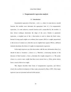
where p is the dimension, 1 is a p-dimensional vector of ones, and is a covariance matrix with the off-diagonal entries set to .8 and the diagonal entries set to 1. These functions will be referred to, respectively, as Linear, Gaussian, Correlated Gaussian, Mixture, and Product. Figure 1 shows graphical representations of bivariate versions of these functions (i.e., two explanatory variables and one response variable). Dimension. The three levels of this factor take the dimension of the explanatory variable space to be p = 2; 6; 12.

4

Linear

Gaussian

Mixture

Correlated Gaussian

Product

Figure 1: Graphical representations of bivariate versions of the functions used in the simulation experiment (i.e., two explanatory variables and one response variable).

k= 4 k = 10 k = 25

p = 2 p = 6 p = 12 16 40 100

256 16,384 640 40,960 1,600 102,400

Table 1: Values of n for different values of dimension (p = 2; 6; 12) for small (k = 4), medium (k = 10), and large (k = 25) sample sizes. Sample size. The three levels of this factor take the sample size to be n = 2p k , where p is the dimension and k = 4; 10; 25. This scales across dimension, so that the different values of k correspond to small, medium, and large samples, respectively. Table 1 shows the specific values of n for different values of p and k . Noise. This factor determines the variance in the additive Gaussian error associated with each observation. The standard deviations of the error variance are = 0:02; 0:1; 0:5. Model sparseness. This factor determines the proportion of explanatory variables that are functionally related to the response variable. The different levels consist of all variables, half of the variables, and none of the variables. When none of the variables are explanatory, then the Constant function f ( i ) = 1:0 is used regardless of the level of the Function factor.

X

Note that not all combinations of this design are realizable. Specifically, when model sparseness is set so that none of the variables pertain to the response variable, then the level of function is 5

irrelevant. Also, LOESS, neural networks, and sometimes AVAS required too much memory or time when the sample size and/or dimension factors were large, resulting in additional missing combinations. These issues will manifest in the results reported in Section 4 and in Appendix A. For a particular combination of factor levels, the simulation experiment proceeds as follows: 1. Generate a uniform random sample

X ; : : :; X n inside the unit hypercube in IRp.

2. Generate a sample of random errors (iid) N (0; 2).

1

1; : : : ; n, all independent and identically distributed

X

3. Calculate Yi = f ( i ) + i , where f : IRp ! IR is the target function determined by appropriate combinations of levels of function, dimension, and model sparseness. 4. Apply the regression method to obtain fˆ, an estimate of f . 5. Estimate the integrated squared error of fˆ over the unit cube (via Monte Carlo, on 10,000 random uniform points). Call this M .

6. Repeat the first five steps 20 times. The average of the 20 resulting M values is an estimate of the MISE; the standard error of this estimate is also calculated for use in subsequent comparisons. Both the random data sample and the Monte Carlo integration sample were reused for all regression methods. These variance reduction techniques improve the accuracy of contrasts between the methods. From each combination of factor levels, an estimate of the MISE and its standard error was obtained. Regression methods whose MISE values are significantly lower than competing methods are superior. Note, however, that the COD implies that values of M for large p are less accurate than for smaller p (with all other factors remaining constant); this needs to be taken into account when interpreting the results. The goal is to understand which regression methods are best for which levels (or combinations of levels) of function, dimension, model sparseness, sample size, and noise.

3.1.

Regression methods

Multiple linear regression (MLR) and stepwise linear regression (SLR) are standard methods that have been used for decades. These methods are included as performance benchmarks for the simulation study; it is assumed that most readers are already familiar with both techniques. For MLR and SLR, the experiment used the commercial code available from SAS, with the SAS defaults for entering and removing variables in SLR (i.e., using the SELECTION=STEPWISE option of PROC REG). A study of SLR performance is given by Frank and Friedman (1993). For the remaining regression techniques, the simplest options and defaults were used consistently: the fitted models were not primed to include polynomial or product terms, MARS and LOESS 6

made first-order fits, and settings did not vary from one level of function to another. (Readers who want details on the smoothers used by the regression methods and the default parameter settings should examine the corresponding documentation.) The code for the regression techniques used in the experiment (with the exception of MLR and SLR) was assembled into a package called DRAT (Data Regression via Assembled Techniques); the DRAT package is available at ftp://ftp.cs.cmu.edu/user/bobski/drat/. 3.1.1. Additive model The additive model (AM) has been developed by several authors; Buja, Hastie and Tibshirani (1989) describe the background and early development. The simplest AM has the form

p X

E[Yi ] = 0 +

j =1

fj (Xij )

(1)

where the functions fj are unknown. Since the fj are estimated from the data, one avoids the traditional assumption of linearity in the explanatory variables; however, AM retains the assumption that explanatory variable effects are additive. Thus the response is modeled as the sum of arbitrary smooth univariate functions of the explanatory variables, but not as the sum of multivariate functions of the explanatory variables. One needs a reasonably large sample size to estimate each fj , but under the model posited in Equation (1), the sample size requirement grows only linearly in p. The backfitting algorithm, described in Hastie and Tibshirani (1990), is the key procedure used to fit an AM: it is guaranteed to find the best fit between a given model and the data. Operationally, the backfitting algorithm proceeds as follows: 1. At the initialization step, define functions fj

(0)

2. At the ith iteration, estimate fj(i+1) by

fj i

( +1)

for j

=

=

Sm(Y , 0 ,

1 and set 0 = Y¯ . X i fk k= 6 j

j X1j ; : : :; Xnj )

1; : : :; p.

3. Check whether jfj(i+1) , fj(i) j < for all j = 1; : : :; p, where is the convergence tolerance. If not, return to step 2; otherwise, use the fj(i) as the additive functions fj in the model. This algorithm requires a smoothing operation (such as kernel smoothing or nearest-neighbor averaging), indicated by Sm( j ). For large classes of smoothing functions, the backfitting algorithm converges to a unique solution. 7

3.1.2. Projection pursuit regression The AM considers sums of functions taking arguments in the natural coordinates of the space of explanatory variables. When the underlying function is additive with respect to variables formed by linear combinations of the original explanatory variables, the AM is inappropriate. Projection pursuit regression (PPR) was designed by Friedman and Stuetzle (1981) to handle such cases. PPR employs the backfitting algorithm and a conventional numerical search routine, such as GaussNewton, to fit a model of the form r X fk ( Tk i) E[Yi ] = k =1

X

where the 1; : : : ; r determine a set of r linear combinations of the explanatory variables. These linear combinations are analogous to those used in principal components analysis (cf. Flury, 1988). A salient difference is that these vectors need not be orthogonal; they are chosen to maximize the predictive accuracy of the model as assessed through generalized cross-validation. Specifically, the PPR alternately calls two routines. The first conditions upon a set of pseudovariables that are linear combinations of the original variables; these are used in the backfitting algorithm to find an AM that sums functions whose arguments are the pseudovariables (which need not be orthogonal). The second routine conditions upon the estimated AM functions, and searches for linear combinations of the original variables that maximize the fit. Alternating iterative application of these methods converges, very generally, to a unique solution. PPR can be hard to interpret when r > 1. If r is allowed to grow without bound, PPR is consistent. Unlike AM, PPR is invariant to affine transformations of the data; this is appealing when the measurements impose no natural basis. 3.1.3. Recursive partitioning regression Recursive partitioning regression (RPR) methods have become popular since the advent of the CART (Classification And Regression Trees) methodology, developed by Breiman, Friedman, Olshen and Stone (1984). This project is concerned with regression problems, in which the basic RPR algorithm fits a model of the form E[Yi ] =

M X j =1

j IRj (X i)

X i) is an indicator

where the R1 ; : : :; RM are rectangular regions that partition IRp , and IRj ( function taking the value 1 if and only if i 2 Rj , and otherwise is zero.

X

RPR is designed to be very good at finding local low-dimensional structure in functions that show high-dimensional global dependence. It is consistent and has a powerful graphic representation as a decision tree which increases interpretability. However, many elementary functions are awkward for RPR, and it is difficult to discover when the fitted piecewise-constant model 8

approximates a standard smooth function. The RPR code available on Statlib (accessible at http://lib.stat.cmu.edu/) was used, rather than CART, to enable inclusion of nonproprietary code in DRAT. 3.1.4. Multivariate adaptive regression splines Friedman (1991a) describes a method that combines the PPR with RPR, using multivariate adaptive regression splines. This procedure fits a weighted sum of multivariate spline basis functions, also known as tensor-spline basis functions, and the model takes the form q X E[Yi ] = ak Bk (X1 ; : : : ; Xn) k =0 where the coefficients ak are determined in the course of generalized cross-validation fitting. The constant term follows by setting B0 (X1 ; : : :; Xn ) 1, and the other multivariate splines are products of univariate spline basis functions: rk Y Bk (x1 ; : : :; xn) = b(xi(s;k)jts;k ) 1kr s=1

Here the subscript i(s; k ) indicates a particular explanatory variable, and the basis spline in that variable has a knot at ts;k . The values of q , the r1; : : : ; rq , the knot sets and the appropriate explanatory variables for inclusion are all determined adaptively from the data. Multivariate adaptive regression splines (MARS) admits an ANOVA-like decomposition that can be represented in a table and similarly interpreted. MARS is designed to perform well whenever the true function has low local dimension. The procedure automatically accommodates interactions between variables and variable selection. 3.1.5. Alternating conditional expectations Another extension of AM permits functional transformation of the response variable, as well as the p explanatory variables. The alternating conditional expectations (ACE) algorithm, developed by Breiman and Friedman (1985), fits the model E[g (Yi )] = 0 +

p X j =1

fj (Xij )

(2)

where all conditions are as given for Equation (1), except g is an unspecified function, scaled to satisfy the technically necessary constraint that var[g (Y )] = 1 (otherwise, the zero transformation would be trivially perfect).

X i] , Ppj fj (Xij )

X

Given variables Yi and i , one wants g and f1 ; : : :; fp such that E[g (Yi )j resembles independent error (without loss of generality, the constant term 9

=1

0 can be ignored).

Formally, one solves

8 2 32 9 > > p n > : i=1 ; j =1 where gˆ satisfies the unit variance constraint. Operationally, one proceeds as follows: 1. Estimate g by g (0), obtained by applying a smoother to the Yi values and standardizing the (0) variance. Set fj 1 for all j = 1; : : :; p. 2. Conditional on g (k,1) (Yi ), apply the backfitting algorithm to find estimates f1(k) ; : : : ; fp(k) . (k ) 3. Conditional on the sum of f1 ; : : :; fp(k) , obtain g (k) by applying the backfitting algorithm (this interchanges the role of the explanatory and response variables). Standardize the new function to have unit variance.

4. Test whether e(k) , e(k,1)

=

ek

( )

If it is zero, set gˆ

=

0, where =

n ,1 X

n

i=1

2 32 p X ( k ) 4g (k) (Yi ) , fj (Xij )5 j =1

g k , fˆj = fj k ; otherwise, go to step 2. ( )

( )

Steps 2 and 3 calculate smoothed expectations, each conditional upon functions of either the response or the explanatory variables; this alternation gives the method its name. The ACE analysis finds sets of functions for which the linear correlation of the transformed response variable and the sum of the transformed explanatory variables is maximized. Thus ACE is closer kin to correlation analysis, and the multiple correlation coefficient, than to regression. Since ACE does not aim directly at regression, it has some undesirable features; for example, it treats the response and explanatory variables symmetrically, small changes can lead to radically different solutions (cf. Buja and Kass, 1985), and it does not reproduce model transformations. To increase fairness of comparison, the experiment used an implementation of ACE slightly modified to include a stepwise selection rule mimicking that of SLR. 3.1.6. Additivity and variance stabilization To overcome some of the potential drawbacks of the ACE methodology, Tibshirani (1988) invented a variation called additivity and variance stabilization (AVAS), which imposes a variance-stabilizing transformation in the ACE backfitting loop for the explanatory variables. AVAS avoids at least two of the deficiencies of ACE in regression applications: it reproduces model transformations and it removes the symmetry between response and explanatory variables. 10

3.1.7. Locally weighted regression Cleveland (1979) proposed a locally weighted regression (LOESS) technique. Rather than simply taking a local average, LOESS fits a model of the form E[Y ] = ( )T where

x x

n

ˆ (x) = argmin2IRp X wi(x)(Yi , TX i )

2

i=1

and wi is a kernel function that weights the influence of the ith observation according to the (oriented) distance of i from .

X

x

Cleveland and Devlin (1988) generalize LOESS to include polynomial regression, rather than just multiple linear regression, in fitting Yi to the data, but the improvement seems small. LOESS has good consistency properties, but can be inefficient at discovering some relatively simple structures in data.

3.1.8. Neural networks Many neural network (NN) techniques exist, but from a statistical regression standpoint (cf. Barron and Barron, 1988), nearly all variants fit models that are weighted sums of sigmoidal functions whose arguments involve linear combinations of the data. A typical feed-forward network uses a model of the form m X E[Y ] = 0 + if ( Ti + i0 ) i=1 where f () is a logistic function and the 0, i0 , and i are estimated from the data. Formally, this approach is similar to that in PPR. The choice of m determines the number of hidden nodes in the network, and affects the smoothness of the fit; in most cases the user determines this parameter, but for the experiment, m is also estimated from the data.

x

The particular implementation of the neural net strategy that was employed is Cascor, developed by Fahlman and Lebiere (1990) and used in a similar large-scale simulation comparison of classification methods, described in Sutherland et al. (1993). It was chosen because it learns more rapidly than standard feedforward nets with backpropagation training, because it was used previously in a major comparison, and because it adaptively chooses the number of hidden nodes, thereby making the analysis more automatic. However, Cascor is not necessarily a good indicator of all neural network strategies. Recent work (Doering, Galicki, and Witte, 1997) suggests that in some cases Cascor does not find optimal weights, and thus some alternative implementation of neural net methods may achieve better performance. Neural nets are widely used, although their performance properties, compared to alternative regression methods, have not been thoroughly studied. Ripley (1993) describes one assessment which finds that neural net methods are not generally competitive. Another difficulty with neural nets is that the resulting model is hard to interpret.

11

3.2.

Other design considerations

The other factors used in the simulation experiment (i.e., function, dimension, sample size, noise, and model sparseness) reflect conventional criteria for performance comparison. Only a few comments seem necessary: Function. The different levels of function were chosen to reflect the range of structure that practitioners typically encounter in applications. As shown in Figure 1, these include essentially flat surfaces (Linear), surfaces with one or more bumps (Gaussian and Correlated Gaussian), surfaces with structure that is additive in either the natural explanatory variables or linear combinations of them (Mixture), and surfaces that incorporate multiplicative interactions (Product). Also, these choices exercise each of the methods; by their constructions, ACE and AVAS should excel on the Product function, NN and PPR should do well on the Correlated Gaussian function, LOESS and AM should handle the Gaussian function, and RPR and MARS should do well with the Mixture function. Dimension. The values taken by the dimension factor may seem small. However, previous experience with the impact of the curse of dimensionality (COD) suggests that this is the correct arena for comparing the different methods. In higher dimensions, all methods perform so poorly that comparison is difficult. Sample size and noise. The values of the sample size and noise factors are typical of previous simulation studies. Qualitatively, these two effects are similar, since a large sample with large noise is informationally comparable to a smaller sample with smaller noise. Model sparseness. Variable selection is a key concern, both in practice and in theory. Including the model sparseness factor enables users to assess the regression methods with respect to this. But the automatic selection rules may not be comparable across implementations, and thus our results compare default performances, rather than the best that an expert might coax by tuning. The guiding principle behind the choice of these factor levels is to explore the range of situations that arise in applications, and thereby assist practitioners who have some prior sense of the kinds of regression structures they face.

4. Results The results of the study consist of the estimated MISE and its variance for 10 5 34 different situations (less a few, since (1) when model sparseness sets all variables to be spurious, the function level becomes irrelevant, and (2) some programs took several days to run, or exhausted the available memory on the computer, with large dimensions and/or sample sizes). These data are complex, and are reported in several ways. 12

Noise

n

Var. Expl.

Method

MOD MOD MOD MOD MOD MOD MOD MOD MOD MOD MOD MOD MOD MOD MOD MOD MOD MOD MOD MOD

SMALL SMALL SMALL SMALL SMALL SMALL SMALL SMALL SMALL SMALL SMALL SMALL SMALL SMALL SMALL SMALL SMALL SMALL SMALL SMALL

ALL ALL ALL ALL ALL ALL ALL ALL ALL ALL HALF HALF HALF HALF HALF HALF HALF HALF HALF HALF

MLR SLR ACE AM MARS RPR PPR LOESS AVAS NN MLR SLR ACE AM MARS RPR PPR LOESS AVAS NN

MISE p=2 (27.95) (32.14) 53.12 (27.91) 158.23 1248.37 55.08 59.50 79.40 124.03 27.95 (23.23) 42.42 27.68 (17.99) 1821.76 35.31 59.50 74.93 103.08

St. Err. 7.02 10.65 7.36 7.01 35.32 307.78 13.14 9.12 18.14 13.05 7.02 6.75 5.92 7.00 3.24 64.32 5.61 9.12 14.13 8.41

MISE p=6 (3.00) (3.00) 15.06 (3.00) 18.36 176.32 19.24 9.14 14.73 100.42 3.00 (2.39) 14.58 3.00 11.00 239.41 13.95 9.14 15.02 94.92

St. Err.

p = 12

MISE

St. Err.

.26 .26 1.14 .26 1.88 10.89 8.68 .52 .95 2.43 .26 .30 1.12 .26 1.68 4.50 8.09 .52 1.08 2.65

(.09) (.09) .41 (.09) .30 61.53 .11 * .38 * (.09) (.08) .40 (.09) .40 100.04 .11 * .36 *

.01 .01 .02 .01 .02 .78 .01 * .02 * .01 .01 .02 .01 .02 2.47 .01 * .01 *

Table 2: A subset of the results for the case where function is Linear, sample size is small (k = 4), and noise is moderate ( = 0:1). Dimension level is indicated by p. All numbers have been multiplied by 10,000. Asterisks denote cases in which no data were available. The parenthesized MISE values were not significantly different from the best regression method under a two-sample t-test with = :05. Table 2 gives a subset of the results for the case where function is Linear, sample size is small (k = 4), and noise is moderate ( = 0:1); the MISE values have been multiplied by 10,000 for ease of reading. Much of this information is later expressed in Figure 3, where these MISE values are the data points in each of the six graphs for the case where sample size is small. (The complete set of results is reported in Appendix A; the subset shown in Table 2 appears on page 30.) A more powerful comparison could be made by taking account of the variance reduction induced by the sample reuse; in that case, most of the MISE values are significantly different, and the method with minimum MISE is strongly favored. But that degree of scrutiny ensures that “Le mieux est l’ennemi du bien;” it seems better service to highlight all methods that work well, rather than to emphasize one that is marginally best. When one has little information about the application, a method that never does badly may be preferred to one that is sometimes the best, but sometimes among the worst. The overall performance of the competing regression methods can be ascertained by taking the ratio of the MISE for a given method to the MISE for the best method, for each combination of factor levels, and then averaging 13

Method MLR SLR ACE AM MARS RPR PPR LOESS AVAS NN

p = 2 p = 6 p = 12 2.40 3.21 1.77 1.70 7.49 30.43 2.49 4.68 1.08 15.86 39.38 21.92 6.71 14.53 4.85 9.74 7.77 26.83 28.46 644.08

15.03 8.35 165.70 29.58 72.58 1.00 41.20 * 97.07 *

Table 3: Averages of the MISE ratios for each regression method, broken out by dimension level (indicated by p), for the case where model sparseness sets all variables to be spurious (i.e., the Constant function was used regardless of function level). Averages were taken over the noise and sample size levels. Asterisks denote cases in which no data were available.


All Explanatory p = 2 p = 6 p = 12 1.00 1.00 1.00 1.12 1.10 1.13 5.07 5.95 5.35 1.00 1.01 1.00 2.57 5.57 8162.43 782.77 1053.40 22217.08 4.11 3.59 1.45 1.94 2.98 * 11.25 5.95 4.51 22.11 96.85 *

Half Explanatory p = 2 p = 6 p = 12 1.19 1.27 1.08 1.04 1.00 1.00 4.20 7.17 5.71 1.22 1.29 2.19 1.73 6.92 300.42 2536.65 3049.21 36891.63 3.13 4.11 1.55 2.29 3.80 * 6.67 7.02 4.70 44.95 157.34 *

Table 4: Averages of the MISE ratios for each regression method, broken out by dimension (indicated by p) and model sparseness levels, for the case where function is Linear. Averages were taken over the noise and sample size levels. Asterisks denote cases in which no data were available.

14

Method

All Explanatory p = 2 p = 6 p = 12 MLR 4.10 2.02 7.51 SLR 4.15 1.91 4.40 ACE 2.84 6.73 75.19 AM 4.10 2.02 7.51 MARS 1.91 4.82 34.71 RPR 49.37 12.31 1.01 PPR 2.89 3.56 19.16 LOESS 1.27 2.43 * AVAS 3.71 6.25 17.39 NN 8.06 92.55 *


Table 5: Averages of the MISE ratios for each regression method, broken out by dimension (indicated by p) and model sparseness levels, for the case where function is Gaussian. Averages were taken over the noise and sample size levels. Asterisks denote cases in which no data were available.

Method



Table 6: Averages of the MISE ratios for each regression method, broken out by dimension (indicated by p) and model sparseness levels, for the case where function is Correlated Gaussian. Averages were taken over the noise and sample size levels. Asterisks denote cases in which no data were available.

15

Method



Table 7: Averages of the MISE ratios for each regression method, broken out by dimension (indicated by p) and model sparseness levels, for the case where function is Mixture. Averages were taken over the noise and sample size levels. Asterisks denote cases in which no data were available.


All Explanatory p = 2 p = 6 p = 12 2.69 8.96 16.66 2.78 9.02 16.67 2.13 1.74 1.01 2.69 8.96 16.67 1.81 4.70 57.66 36.30 31.70 61.11 3.27 9.39 16.24 1.20 7.14 * 3.81 3.35 5.25 6.40 20.96 *


Table 8: Averages of the MISE ratios for each regression method, broken out by dimension (indicated by p) and model sparseness levels, for the case where function is Product. Averages were taken over the noise and sample size levels. Asterisks denote cases in which no data were available.

16

these ratios over the levels of noise and sample size. Table 3 shows this analysis for the case where model sparseness sets all variables to be spurious (i.e., the Constant function was used regardless of function level); the results are broken out by dimension levels. Tables 4, 5, 6, 7, and 8 show this analysis for the cases where function is set, respectively, to Linear, Gaussian, Correlated Gaussian, Mixture, and Product; the results are broken out by dimension and model sparseness levels. Asterisks denote cases in which no data were available. This tabular information is difficult to apprehend; graphs enable a stronger sense of comparison. To that end, two figures are shown, all for the moderate level of noise ( = 0:1), that describe the performance of the methods across dimension and sample size levels. The figures do not include error bars, since (1) this would complicate the images, and (2) the error bars could not take account of the variance reduction attained by sample reuse. The correlation between most methods is very high, and thus visually distinct curves may safely be regarded as statistically distinct. First consider the case when all explanatory variables are spurious. Here the best predictive rule is IE[y ], but many methods overfit. Figure 2 shows the relationship among the methods that attained the smallest MISE. Again, to simplify the graph labels, the MISE has been multiplied by 10,000. Table 9 provides a key for associating regression techniques with the lines on the graphs in Figure 2: the regression techniques are ordered in the table for each graph according to their position when sample size is small. For example, the graph lines in the middle graph of Figure 2, from better to worse MISE (i.e., from smaller to larger MISE values) for the small sample size, are associated with the regression methods are SLR, MLR and AM (i.e., the graph lines for MLR and AM are indistinguishable), LOESS, PPR, MARS, AVAS, ACE, and RPR. Methods not shown have such large MISEs that their inclusion would compress the scale among the good performers, making visual distinctions difficult. Note that the MISE values typically decrease with dimension, suggesting that the increase in sample size to match the level of dimension is too generous. But cross-dimensional comparisons are not straightforward, since MISE is not a dimensionless quantity (cf. Scott, 1992). Within the dimension levels, RPR does very well when dimension is high (p = 12), and badly otherwise; MARS does well when dimension is low (p = 2), and degrades for larger values of dimension. SLR, MLR, and AM are consistently competitive. The theoretical minimum that the optimal procedure could be expected to attain is 104 2=2p k , where = :1 and p and k are determined by the dimension and sample size levels. For low dimension (p = 2), some methods come close to this bound; for larger p, the curse of dimensionality is apparent. Figure 3 shows six graphs for the case where function is Linear: the lefthand column pertains to the case where model sparseness sets all variables to be explanatory, and the righthand column pertains to the case where model sparseness sets half the variables to be explanatory. As before, all MISE values are multiplied by 10,000. Table 10 provides a key for associating regression techniques with the lines on the graphs in Figure 3: the regression techniques are ordered in the table for each graph according to their position when sample size is small. For example, the graphs lines in the top left of Figure 3, from better to worse MISE (i.e., from smaller to larger MISE values) for the small sample size, are associated with the regression methods MLR and AM (i.e., the graph lines for MLR and AM are indistinguishable), SLR, PPR, AVAS, ACE. As before, methods with very large MISEs are not included, to enhance visual resolution of comparative performance. 17

MISE

60

MISE

25

MISE

1.00

20 0.75

45 15

0.50

30 10

0.25

15 5

0.00 Small

Medium

Large Sample Size

High Dimension

0 Small

Medium

Large Sample Size

0 Small

Medium Dimension

Medium

Large Sample Size

Low Dimension

Figure 2: Graphs of MISE values for the case where model sparseness sets all variables to be spurious (i.e., the Constant function was used regardless of function level), broken out by dimension and sample size levels. Each line connects the MISE values for a particular regression method. All MISE values have been multiplied by 10,000. The key to associate regression techniques with graph lines is in Table 9.

ACE AVAS MARS PPR AM MLR SLR RPR High Dimension

Larger MISE

6 ?

Smaller MISE

RPR ACE AVAS MARS PPR LOESS MLR,AM SLR Medium Dimension

Larger MISE

6 ?

Smaller MISE

LOESS ACE AVAS PPR MLR,AM SLR MARS Low Dimension

Table 9: The key to associate regression techniques with lines on the graphs in Figure 2. This table is laid out in blocks, similar to the graphs in the figure. Each block in the table lists the regression techniques associated with the lines of the corresponding graph for the case of small sample size.

18

High Dimension

MISE

0.50

MISE

0.50

0.40

0.40

0.30

0.30

0.20

0.20

0.10

0.10

0.00 Small

Medium

Large Sample Size

Medium Dimension

Large Sample Size

Medium

Large Sample Size

Medium

Large Sample Size

MISE

15

15

10

10

5

5

0 Small

Medium

0 Small

Large Sample Size

MISE

80

MISE

80

Low Dimension

Medium

20

MISE

20

0.00 Small

60

60

40

40

20

20

0 Small

Medium

Large Sample Size

None

0 Small

Half

Proportion of Spurious Variables Figure 3: Graphs of MISE values for the cases where model sparseness sets all variables to be explanatory (lefthand column) and half the variables to be explanatory (righthand column), broken out by dimension and sample size levels. Each line connects the MISE values for a particular regression method. All MISE values have been multiplied by 10,000. The key to associate regression techniques with graph lines is in Table 10.

19

High Dimension

ACE AVAS PPR SLR MLR,AM

Larger MISE

6 ?

Smaller MISE

Larger MISE

Medium Dimension

6

PPR MARS ACE AVAS LOESS MLR,SLR,AM

?

Smaller MISE

Larger MISE

Low Dimension

6

AVAS LOESS PPR ACE SLR MLR,AM

?

Smaller MISE

None

ACE AVAS PPR MLR,AM SLR AVAS ACE PPR MARS LOESS MLR,AM SLR AVAS LOESS ACE PPR MLR,AM SLR MARS Half

Proportion of Spurious Variables Table 10: The key to associate regression techniques with lines on the graphs in Figure 3. This table is laid out in blocks, similar to the graphs in the figure. Each block in the table lists the regression techniques associated with the lines of the corresponding graph for the case of small sample size.

20

Unsurprisingly, MLR excels in the left column, and SLR in the right. The overall shapes of the lines within graphs are consistent with increasing sample size, except for the the odd performance of MARS in the lower right graph. It appears MARS has been tuned, during its design, to handle this paradigm situation when dimension is low (p = 2). More generally, the tables indicate that MARS shows marked variability in performance for linear functions; this is reasonable, since its design employs local linear fits. When all knots are removed, one supposes that MARS acts like SLR; but when some knots, by chance, persist, then MARS cannot employ the global information available to SLR, MLR, AM, PPR, ACE, or AVAS. Within dimension, the graphs for the two levels of model sparseness are quite similar. This suggests that the variable-selection overhead roughly cancels the advantage from fitting a simpler model. Presumably this correspondence would weaken if the numbers of independent variables or the levels of dimension were changed. Similar figures (not shown here) for the other function levels typically have larger MISE values, and show pronounced differences between the two levels of model sparseness. The insights drawn from these other figures are reflected in the discussion in Section 5.

5. Conclusions The tables and figures shown or alluded to in Section 4 describe, for different types of functions, the performance of the regression methods under examination. A reverse index is now presented: the performance of each method in different situations is summarized.

MLR, SLR, and AM perform similarly over all situations considered, and represent broadly safe choices. They are never disastrous, though rarely the best (except for MLR when the function is Linear and all variables are explanatory). For the Constant function, SLR shows less overfit than MLR, which is better than AM; however, it is easy to find functions for which AM would outperform both MLR and SLR. SLR is usually slightly better with spurious variables, but its strategy becomes notably less effective as the number of spurious variables increases, especially for non-linear functions. All three methods have greatest relative difficulty with the Product function, which has substantial curvature. On theoretical grounds ACE and AVAS should be similar, but this is not always borne out. ACE is decisively better for the Product function, and AVAS for the Constant function. ACE and AVAS are the best methods for the Product function (as expected—the log transformation produces a linear relationship), but among the worst for the Constant function and for the Mixture function; in other cases, their performance is not remarkable. Both methods are fairly robust to spurious variables. Contrary to expectation, MARS does not show well in higher dimensions, especially when all variables are explanatory, and especially for the Linear function. However, for lower levels of dimension, MARS shows adequate performance across the different function levels. 21

p=2

p=6

p = 12

All Explanatory Linear MLR,SLR Gaussian LOESS,MARS Correlated Gaussian LOESS Mixture LOESS Product ACE

MLR,SLR SLR LOESS,NN LOESS ACE

MLR,SLR RPR ACE,AVAS RPR ACE

Half Explanatory Linear Gaussian Correlated Gaussian Mixture Product None Explanatory

MLR,SLR MLR,SLR MLR,SLR MARS,PPR MARS,PPR MARS,PPR MARS MARS MARS MARS MARS MARS ACE ACE ACE MARS

SLR

RPR

Table 11: The most effective regression technique(s) for each combination of dimension (indicated by p), number of explanatory variables, and underlying functional relationship. MARS is well-calibrated for the Constant function when p = 2, but finds spurious structure for larger values, which may account for some of its failures.

RPR was consistently bad in low levels of dimension, but sometimes stunningly successful in high levels of dimension, especially when all variables were explanatory. Surprisingly, its variable-selection capability was not very successful (MARS’s implementation clearly outperforms it). Perhaps the CART program, with its flexible pruning, would surpass RPR, but previous experience with CART suggests such an improvement is dubious. Unsurprisingly, RPR’s design made it uncompetitive on the Linear function. PPR and NN are theoretically similar methods, but PPR was clearly superior in all cases except for the Correlated Gaussian function. This may reflect peculiarities of the Cascor implementation of neural nets. PPR was often among the best when the function was Gaussian, Correlated Gaussian, or Mixture, but among the worst with the Product function and when all variables were spurious. PPR’s variable selection was generally good. In contrast, NN was generally poor, except for the Correlated Gaussian function when p = 2; 6 and all variables are explanatory and when p = 6 and half the variables are explanatory. The Correlated Gaussian function lends itself to approximation by a small number of sigmoidal functions whose orientations are determined by the data. LOESS does well in low levels of dimension with the Gaussian, Correlated Gaussian, and Mixture function. It is not as successful with the other function levels, especially the Constant function. Often, it is not bad in higher levels of dimension, though its relative performance tends to deteriorate. 22

Additional comparative observations on performance are:

For the Constant function, MARS is good when p = 2, SLR is good when p = 6, and RPR is good when p = 12. For the Linear function, MLR and SLR are consistently strong. For the Gaussian function, with all variables explanatory, LOESS and MARS are good when p = 2, SLR is good when p = 6, and RPR is good when p = 12; when half of the variables are explanatory, MARS and PPR perform well. For the Correlated Gaussian function, with all variables explanatory, LOESS works well for p = 2, LOESS and NN for p = 6, and ACE or AVAS for p = 12; with half the variables explanatory, MARS is reliably good. For the Mixture function, with all variables explanatory, LOESS works well for p 6, and RPR for p = 12; with half of the variables explanatory, MARS is consistently good. There is considerable variability for the product function, but ACE is broadly superior. Table 11 summarizes these observations. Two kinds of variable-selection strategies were used by the methods: global variable selection, as practiced by SLR, ACE, AVAS, and PPR, and local variable reduction, as practiced by MARS and RPR. Generally, the latter does best in high levels of dimension, but performance depends on the level of function. LOESS, NN, and sometimes AVAS proved infeasible in high levels of dimension. The number of local minimizations in LOESS grew exponentially with p. Cascor’s demands were high because of the cross-validated selection of the hidden nodes; alternative NN methods fix these a priori, making fewer computational demands, but this is equivalent to imposing strong, though complex, modeling assumptions. Typically, fitting a single highdimensional dataset with either LOESS or NN took more than two hours. AVAS was faster, but the combination of high dimension and large sample size also required substantial time.

These findings are broadly consistent with those of previous authors, but perhaps more comprehensive.

6. Summary To restate the most important conclusions, MLR, SLR, and AM are blue-chip methods, that rarely do badly. When the response function is rough, they tend to fit the average, which is often a sensible default. Obviously, a method that in the same circumstances tended to fit the median might have more attractive robustness properties. NN is unreliable; it can do well, but most often has very large MISE compared to other methods. (Part of this may be that Cascor is not an effective implementation of neural net strategy.) The only cases in which NN was decently competitive were the Correlated Gaussian function with p = 2; 6 and all variables explanatory, and p = 6 with half of the variables explanatory. However, in practice, NN methods are reported to be very effective. One conjecture is that this is because 23

for many applications, the response function has a sigmoidal shape over the domain of interest, as happened in the example with the Correlated Gaussian function. MARS is less able in higher dimensions than recent enthusiasm suggests, but it handles a broad range of cases well, and rarely has relatively large MISE. Insofar as MARS combines PPR and RPR strategies, it appears to have protected itself against the worst failures of both, but not attained the best performances of either; such compromise is probably unavoidable. A further hybrid that employs the ACE transformation strategy would potentially be effective. As a final recommendation for practice, analysts are urged to set aside a portion of the original data, and use each of the reasonable methods to predict the holdouts. The method which does the best job in this test ought to be the method of choice for the unknown situation in hand. This obviates the need for strong prior knowledge about the form of the function, and reduces the inclination to engage in philosophical disputes on the merits of competing strategies for multivariate nonparametric regression.

24

A. Complete results of the simulation experiment The following tables contain the complete results from the simulation experiment, broken out by levels of function, noise, sample size (indicated by n), model sparseness, regression method, and dimension (indicated by p). For each combination of factor levels, the MISE and its standard error are reported. All MISE values have been multiplied by 10,000. Asterisks denote cases in which no data were available (the methods took too long to run or had excessive memory demands). When model sparseness sets all variables to be spurious, the Constant function is used regardless of function level. To eliminate redundancy, the results for the case where all variables are spurious appear as their own set of tables for the Constant function, and these results are omitted from the tables for each function level.

25

Function: Constant Noise

n

Var. Expl.

Method

LOW LOW LOW LOW LOW LOW LOW LOW LOW LOW LOW LOW LOW LOW LOW LOW LOW LOW LOW LOW LOW LOW LOW LOW LOW LOW LOW LOW LOW LOW MOD MOD MOD MOD MOD MOD MOD MOD MOD MOD

SMALL SMALL SMALL SMALL SMALL SMALL SMALL SMALL SMALL SMALL MED MED MED MED MED MED MED MED MED MED LARGE LARGE LARGE LARGE LARGE LARGE LARGE LARGE LARGE LARGE SMALL SMALL SMALL SMALL SMALL SMALL SMALL SMALL SMALL SMALL

NONE NONE NONE NONE NONE NONE NONE NONE NONE NONE NONE NONE NONE NONE NONE NONE NONE NONE NONE NONE NONE NONE NONE NONE NONE NONE NONE NONE NONE NONE NONE NONE NONE NONE NONE NONE NONE NONE NONE NONE

MLR SLR ACE AM MARS RPR PPR LOESS AVAS NN MLR SLR ACE AM MARS RPR PPR LOESS AVAS NN MLR SLR ACE AM MARS RPR PPR LOESS AVAS NN MLR SLR ACE AM MARS RPR PPR LOESS AVAS NN

MISE St. Err. MISE St. Err. p=2 p=6 1.12 .28 .12 .01 .83 .28 .07 .01 2.18 .35 .96 .06 1.12 .28 .14 .02 .26 .07 .51 .09 7.17 1.68 3.27 .36 2.03 .27 .47 .05 2.38 .36 .37 .02 2.20 .28 .90 .06 4.57 .49 4.21 .12 .34 .06 .05 .01 .24 .06 .04 .01 1.31 .19 .41 .02 .37 .07 .10 .02 .21 .08 .20 .04 7.30 1.62 .58 .20 1.27 .14 .19 .02 .71 .13 .14 .00 1.46 .19 .37 .03 4.32 .30 4.20 .08 .13 .02 .02 .00 .10 .02 .01 .00 .79 .08 .16 .01 .21 .04 .04 .01 .12 .08 .08 .01 5.36 1.49 .00 .00 .60 .05 .08 .01 .21 .02 .05 .00 .79 .10 .14 .01 4.52 .16 4.19 .04 27.95 7.02 3.00 .26 20.81 6.93 1.68 .30 54.54 8.83 23.91 1.46 27.75 6.99 3.08 .29 6.62 1.74 12.77 2.25 178.52 42.19 81.75 8.87 51.49 6.54 9.91 1.17 59.50 9.12 9.14 .52 53.41 6.95 23.02 1.47 117.30 11.59 102.09 2.33

26

MISE St. Err. p = 12 .00 .00 .00 .00 .04 .00 .01 .00 .02 .00 .00 .00 .01 .00 * * .02 .00 * * .00 .00 .00 .00 .01 .00 .00 .00 .01 .00 .00 .00 .00 .00 * * .01 .00 * * .00 .00 .00 .00 .01 .00 .00 .00 .00 .00 .00 .00 .00 .00 * * .00 .00 * * .09 .01 .05 .01 .87 .05 .11 .02 .48 .03 .00 .00 .23 .02 * * .63 .02 * *

Function: Constant (Cont.) Noise

n

MOD MOD MOD MOD MOD MOD MOD MOD MOD MOD MOD MOD MOD MOD MOD MOD MOD MOD MOD MOD HIGH HIGH HIGH HIGH HIGH HIGH HIGH HIGH HIGH HIGH HIGH HIGH HIGH HIGH HIGH HIGH HIGH HIGH HIGH HIGH

MED MED MED MED MED MED MED MED MED MED LARGE LARGE LARGE LARGE LARGE LARGE LARGE LARGE LARGE LARGE SMALL SMALL SMALL SMALL SMALL SMALL SMALL SMALL SMALL SMALL MED MED MED MED MED MED MED MED MED MED

Var. Expl. Method NONE NONE NONE NONE NONE NONE NONE NONE NONE NONE NONE NONE NONE NONE NONE NONE NONE NONE NONE NONE NONE NONE NONE NONE NONE NONE NONE NONE NONE NONE NONE NONE NONE NONE NONE NONE NONE NONE NONE NONE


MISE St. Err. MISE St. Err. p=2 p=6 8.48 1.38 1.28 .13 6.03 1.52 .90 .14 32.70 4.69 10.31 .63 8.36 1.43 1.30 .14 5.21 2.05 5.03 1.12 181.89 40.63 14.42 5.12 31.38 3.46 4.80 .54 17.67 3.21 3.56 .12 37.31 4.85 9.19 .65 112.31 7.98 105.34 2.31 3.36 .53 .38 .03 2.47 .59 .19 .04 19.65 2.00 3.93 .24 3.32 .55 .45 .04 3.04 1.99 2.06 .25 140.70 37.26 .06 .02 16.26 1.46 1.96 .18 5.34 .53 1.19 .06 19.26 2.52 3.44 .21 113.65 4.70 104.47 1.25 698.86 175.55 75.12 6.58 520.34 173.18 42.09 7.45 1363.56 220.85 597.75 36.47 699.52 175.67 75.38 6.58 165.58 43.50 319.15 56.27 4582.92 1043.68 2060.34 233.91 1287.09 163.50 262.36 19.06 1487.55 227.92 228.57 13.02 1365.34 187.20 567.22 38.60 2979.35 318.09 2656.58 63.22 212.10 34.48 31.89 3.37 150.78 38.06 22.44 3.58 817.43 117.19 257.85 15.66 212.00 34.66 32.06 3.42 130.19 51.14 125.72 27.96 4518.82 1022.41 360.48 128.12 787.15 86.64 104.46 10.07 441.64 80.37 89.01 3.11 905.29 115.21 229.53 16.12 2774.71 203.46 2635.23 55.04 27

MISE St. Err.

p = 12

.03 .02 .35 .05 .16 .00 .09 * .25 * .01 .01 .13 .03 .04 .00 .03 * .04 * 2.13 1.16 21.80 2.15 11.88 .11 5.46 * 15.53 * .76 .45 8.75 .79 3.91 .07 2.11 * 6.41 *

.00 .00 .01 .01 .02 .00 .01 * .01 * .00 .00 .01 .01 .00 .00 .00 * .00 * .25 .26 1.17 .25 .79 .03 .57 * .54 * .06 .07 .29 .07 .46 .03 .16 * .34 *

Function: Constant (Cont.) Noise

n

HIGH HIGH HIGH HIGH HIGH HIGH HIGH HIGH HIGH HIGH

LARGE LARGE LARGE LARGE LARGE LARGE LARGE LARGE LARGE LARGE

Var. Expl. Method NONE NONE NONE NONE NONE NONE NONE NONE NONE NONE

MLR SLR ACE AM MARS RPR PPR LOESS AVAS NN

MISE St. Err. MISE St. Err. p=2 p=6 84.07 13.20 9.62 .75 61.66 14.73 4.67 1.02 491.16 50.03 98.28 5.85 83.76 13.33 9.70 .73 75.95 49.77 51.58 6.14 3496.65 933.24 1.50 .52 388.70 33.36 43.99 2.66 133.52 13.29 29.72 1.49 514.20 62.38 83.33 4.78 2933.91 104.83 2658.15 27.90

28

MISE St. Err.

p = 12 .29 .16 3.35 .33 1.05 .03 .83 * .68 *

.02 .03 .15 .03 .08 .01 .06 * .05 *

Function: Linear Noise

n

Var. Expl.

Method

LOW LOW LOW LOW LOW LOW LOW LOW LOW LOW LOW LOW LOW LOW LOW LOW LOW LOW LOW LOW LOW LOW LOW LOW LOW LOW LOW LOW LOW LOW LOW LOW LOW LOW LOW LOW LOW LOW LOW LOW

SMALL SMALL SMALL SMALL SMALL SMALL SMALL SMALL SMALL SMALL SMALL SMALL SMALL SMALL SMALL SMALL SMALL SMALL SMALL SMALL MED MED MED MED MED MED MED MED MED MED MED MED MED MED MED MED MED MED MED MED

ALL ALL ALL ALL ALL ALL ALL ALL ALL ALL HALF HALF HALF HALF HALF HALF HALF HALF HALF HALF ALL ALL ALL ALL ALL ALL ALL ALL ALL ALL HALF HALF HALF HALF HALF HALF HALF HALF HALF HALF


MISE St. Err. MISE St. Err. p=2 p=6 1.12 .28 .12 .01 1.12 .28 .12 .01 11.08 1.95 .68 .05 1.11 .28 .12 .01 2.19 .43 .48 .05 602.38 85.66 113.45 6.13 9.66 1.82 .30 .03 2.38 .36 .37 .02 29.48 4.91 1.11 .39 21.51 3.15 1.76 .11 1.12 .28 .12 .01 .93 .27 .10 .01 4.57 1.05 .66 .04 1.13 .29 .12 .01 2.11 .65 .46 .08 1651.73 26.01 214.46 3.36 3.86 .98 .29 .02 2.38 .36 .37 .02 16.83 5.73 .86 .05 29.71 2.04 5.19 .45 .34 .06 .05 .01 .34 .06 .05 .01 3.18 .67 .28 .01 .34 .05 .05 .01 .64 .13 .20 .02 627.72 71.44 98.72 2.75 2.37 .56 .12 .01 .71 .13 .14 .00 10.88 2.53 .28 .02 9.93 1.22 1.41 .06 .34 .06 .05 .01 .30 .06 .04 .01 1.75 .33 .26 .02 .41 .07 .05 .01 .64 .13 .20 .02 1636.55 12.22 209.65 2.44 1.18 .28 .11 .01 .71 .13 .14 .00 2.79 .65 .28 .02 24.22 1.80 3.74 .31

29

MISE St. Err. p = 12 .00 .00 .00 .00 .02 .00 .00 .00 .01 .00 57.80 .52 .00 .00 * * .02 .00 * * .00 .00 .00 .00 .02 .00 .00 .00 .02 .00 93.15 1.54 .00 .00 * * .02 .00 * * .00 .00 .00 .00 .01 .00 .00 .00 13.82 1.57 58.43 .81 .00 .00 * * .01 .00 * * .00 .00 .00 .00 .01 .00 .00 .00 .00 .00 90.57 1.90 .00 .00 * * .01 .00 * *

Function: Linear (Cont.) Noise

n

Var. Expl.

Method

LOW LOW LOW LOW LOW LOW LOW LOW LOW LOW LOW LOW LOW LOW LOW LOW LOW LOW LOW LOW MOD MOD MOD MOD MOD MOD MOD MOD MOD MOD MOD MOD MOD MOD MOD MOD MOD MOD MOD MOD

LARGE LARGE LARGE LARGE LARGE LARGE LARGE LARGE LARGE LARGE LARGE LARGE LARGE LARGE LARGE LARGE LARGE LARGE LARGE LARGE SMALL SMALL SMALL SMALL SMALL SMALL SMALL SMALL SMALL SMALL SMALL SMALL SMALL SMALL SMALL SMALL SMALL SMALL SMALL SMALL



MISE St. Err. MISE St. Err. p=2 p=6 .13 .02 .02 .00 .13 .02 .02 .00 .74 .11 .10 .00 .14 .02 .02 .00 .44 .23 .07 .01 560.75 20.64 93.19 1.77 .52 .09 .04 .00 .21 .02 .05 .00 2.76 .67 .09 .01 7.34 .60 1.09 .07 .13 .02 .02 .00 .11 .02 .01 .00 .52 .06 .09 .00 .14 .02 .02 .00 .16 .04 .10 .01 1645.60 8.02 207.54 1.21 .31 .04 .03 .00 .21 .02 .05 .00 .92 .37 .09 .01 20.97 1.41 3.00 .28 27.95 7.02 3.00 .26 32.14 10.65 3.00 .26 53.12 7.36 15.06 1.14 27.91 7.01 3.00 .26 158.23 35.32 18.36 1.88 1248.37 307.78 176.32 10.89 55.08 13.14 19.24 8.68 59.50 9.12 9.14 .52 79.40 18.14 14.73 .95 124.03 13.05 100.42 2.43 27.95 7.02 3.00 .26 23.23 6.75 2.39 .30 42.42 5.92 14.58 1.12 27.68 7.00 3.00 .26 17.99 3.24 11.00 1.68 1821.76 64.32 239.41 4.50 35.31 5.61 13.95 8.09 59.50 9.12 9.14 .52 74.93 14.13 15.02 1.08 103.08 8.41 94.92 2.65 30

MISE St. Err.

p = 12

.00 .00 .00 .00 27.14 58.02 .00 * .00 * .00 .00 .00 .00 1.16 91.64 .00 * .00 * .09 .09 .41 .09 .30 61.53 .11 * .38 * .09 .08 .40 .09 .40 100.04 .11 * .36 *

.00 .00 .00 .00 1.51 .62 .00 * .00 * .00 .00 .00 .00 1.16 1.45 .00 * .00 * .01 .01 .02 .01 .02 .78 .01 * .02 * .01 .01 .02 .01 .02 2.47 .01 * .01 *


n

MOD MOD MOD MOD MOD MOD MOD MOD MOD MOD MOD MOD MOD MOD MOD MOD MOD MOD MOD MOD MOD MOD MOD MOD MOD MOD MOD MOD MOD MOD MOD MOD MOD MOD MOD MOD MOD MOD MOD MOD

MED MED MED MED MED MED MED MED MED MED MED MED MED MED MED MED MED MED MED MED LARGE LARGE LARGE LARGE LARGE LARGE LARGE LARGE LARGE LARGE LARGE LARGE LARGE LARGE LARGE LARGE LARGE LARGE LARGE LARGE

Var. Expl. Method ALL ALL ALL ALL ALL ALL ALL ALL ALL ALL HALF HALF HALF HALF HALF HALF HALF HALF HALF HALF ALL ALL ALL ALL ALL ALL ALL ALL ALL ALL HALF HALF HALF HALF HALF HALF HALF HALF HALF HALF


MISE St. Err. MISE St. Err. p=2 p=6 8.48 1.38 1.28 .13 8.48 1.38 1.28 .13 33.98 3.92 5.94 .23 8.47 1.37 1.28 .13 19.60 4.13 5.54 .52 869.96 103.93 124.07 4.45 26.71 4.34 2.24 .26 17.67 3.21 3.56 .12 36.89 4.44 5.61 .29 99.61 8.50 99.59 2.03 8.48 1.38 1.28 .13 7.38 1.44 1.08 .13 29.42 4.45 5.79 .22 8.52 1.42 1.27 .13 16.73 3.84 5.67 .53 1708.05 41.80 219.15 3.15 18.07 3.28 2.14 .22 17.67 3.21 3.56 .12 33.71 4.57 5.51 .32 97.55 11.51 94.53 1.76 3.36 .53 .38 .03 3.36 .53 .38 .03 13.88 1.15 2.16 .09 3.37 .53 .39 .03 4.35 .67 2.16 .20 828.79 60.61 106.04 3.90 8.31 .90 .82 .07 5.34 .53 1.19 .06 14.87 1.57 1.92 .11 93.48 4.39 99.50 1.05 3.36 .53 .38 .03 2.84 .56 .27 .04 15.45 1.64 2.17 .08 3.38 .52 .38 .03 5.26 1.54 2.41 .34 1671.40 30.36 211.66 2.36 10.49 1.78 .63 .05 5.34 .53 1.19 .06 14.09 1.65 1.91 .10 86.01 5.20 92.99 1.07 31

MISE St. Err.

p = 12 .03 .03 .16 .03 14.45 62.80 .04 * .16 * .03 .03 .16 .03 .10 97.91 .04 * .14 * .01 .01 .06 .01 26.11 61.95 .02 * .03 * .01 .01 .06 .01 1.19 101.42 .02 * .03 *

.00 .00 .01 .00 1.47 .75 .00 * .01 * .00 .00 .01 .00 .01 2.56 .00 * .01 * .00 .00 .00 .00 1.37 .57 .00 * .00 * .00 .00 .00 .00 1.17 2.14 .00 * .00 *


n

HIGH HIGH HIGH HIGH HIGH HIGH HIGH HIGH HIGH HIGH HIGH HIGH HIGH HIGH HIGH HIGH HIGH HIGH HIGH HIGH HIGH HIGH HIGH HIGH HIGH HIGH HIGH HIGH HIGH HIGH HIGH HIGH HIGH HIGH HIGH HIGH HIGH HIGH HIGH HIGH




MISE St. Err. MISE St. Err. p=2 p=6 698.86 175.55 75.12 6.58 853.34 167.67 106.59 5.29 1149.79 161.82 517.59 33.79 700.48 176.17 75.06 6.58 701.76 76.61 458.09 81.63 7167.58 1568.85 2020.65 161.21 1437.90 244.03 337.96 24.76 1487.55 227.92 228.57 13.02 1269.11 184.66 488.20 34.53 2874.32 273.84 2533.64 55.51 698.86 175.55 75.12 6.58 659.82 169.01 65.97 10.33 1306.61 209.63 534.01 38.54 700.57 176.14 75.03 6.56 980.79 99.23 545.75 154.81 6120.10 1335.74 2477.94 304.14 1285.05 255.48 442.21 32.85 1487.55 227.92 228.57 13.02 1243.75 181.84 475.59 37.67 2806.13 347.00 2636.77 69.95 212.10 34.48 31.89 3.37 316.35 40.70 43.89 5.53 870.34 121.43 198.99 10.42 211.72 34.35 31.88 3.37 533.57 40.58 187.33 17.19 5910.82 974.39 720.56 167.88 880.51 125.50 184.61 15.33 441.64 80.37 89.01 3.11 870.12 122.10 178.82 11.76 2919.89 185.31 2585.78 33.27 212.10 34.48 31.89 3.37 231.02 59.73 26.97 3.13 816.30 136.00 180.50 6.83 211.16 34.40 31.89 3.37 406.73 74.99 146.96 20.75 6062.59 941.35 767.26 130.32 674.30 131.88 218.03 27.72 441.64 80.37 89.01 3.11 847.22 128.02 160.28 11.18 2814.44 165.28 2634.68 47.74 32

MISE St. Err.

p = 12

2.13 2.37 11.98 2.13 14.58 69.49 3.64 * 10.27 * 2.13 1.95 10.67 2.14 11.99 137.36 3.04 * 9.62 * .76 .83 4.26 .75 143.64 69.47 1.29 * 4.05 * .76 .67 4.25 .75 2.63 138.27 1.23 * 3.71 *

.25 .21 .68 .25 1.06 .18 .39 * .52 * .25 .22 .52 .25 .47 1.87 .46 * .36 * .06 .08 .18 .06 127.11 .19 .13 * .22 * .06 .08 .21 .06 .17 .36 .10 * .21 *


n

HIGH HIGH HIGH HIGH HIGH HIGH HIGH HIGH HIGH HIGH HIGH HIGH HIGH HIGH HIGH HIGH HIGH HIGH HIGH HIGH

LARGE LARGE LARGE LARGE LARGE LARGE LARGE LARGE LARGE LARGE LARGE LARGE LARGE LARGE LARGE LARGE LARGE LARGE LARGE LARGE

Var. Expl. Method ALL ALL ALL ALL ALL ALL ALL ALL ALL ALL HALF HALF HALF HALF HALF HALF HALF HALF HALF HALF


MISE St. Err. MISE St. Err. p=2 p=6 84.07 13.20 9.62 .75 104.18 18.84 10.10 1.08 416.96 46.59 72.52 3.60 84.05 13.21 9.60 .74 270.37 35.99 92.97 9.55 4472.38 777.70 169.59 11.66 310.89 39.82 41.44 7.12 133.52 13.29 29.72 1.49 385.59 40.45 59.32 4.16 2849.57 94.08 2622.47 21.95 84.07 13.20 9.62 .75 70.99 13.89 6.77 .90 335.56 43.33 62.65 2.91 84.00 13.21 9.61 .74 81.51 17.81 74.02 7.58 4230.49 550.92 268.37 15.27 286.81 24.59 25.29 2.35 133.52 13.29 29.72 1.49 341.80 34.96 52.74 3.40 2771.59 119.81 2641.75 29.16

33

MISE St. Err.

p = 12

.29 .34 1.67 .29 25.72 69.43 .42 * .85 * .29 .28 1.62 .29 .52 138.23 .42 * .79 *

.02 .03 .06 .02 1.20 .18 .03 * .05 * .02 .03 .08 .02 .05 .35 .03 * .05 *

Function: Gaussian Noise

n

Var. Expl.

Method





MISE St. Err. MISE St. Err. p=2 p=6 45.54 2.85 1.73 .02 45.54 2.85 1.73 .02 29.18 4.93 1.75 .06 45.52 2.84 1.72 .02 27.65 5.31 2.30 .14 368.20 25.80 5.54 .39 25.57 2.90 2.29 .32 9.64 1.17 .76 .05 39.62 9.01 1.94 .09 34.29 5.35 5.24 .16 6.83 .35 22.15 .10 6.57 .35 22.06 .11 3.42 .46 5.07 .33 6.85 .36 22.14 .10 5.03 .32 1.47 .07 1060.87 15.00 88.00 1.44 3.11 .52 7.26 .08 6.70 .79 4.82 .15 9.82 3.48 5.62 .47 18.53 1.75 8.72 .50 34.51 .64 1.66 .02 34.51 .64 1.66 .02 9.60 1.48 .98 .05 34.52 .64 1.65 .02 3.73 .34 1.58 .06 378.44 11.40 3.24 .12 14.78 .65 .50 .01 4.06 .41 .52 .02 21.99 2.71 1.14 .06 11.52 1.31 5.00 .10 5.78 .18 21.70 .10 5.68 .18 21.65 .10 1.58 .23 2.32 .10 5.78 .18 21.68 .09 1.97 .25 .91 .04 1046.53 10.33 87.21 .69 1.24 .17 6.53 .05 4.46 .24 3.80 .06 1.71 .23 2.68 .15 13.19 1.47 3.87 .35

34

MISE St. Err. p = 12 .01 .00 .00 .00 .03 .00 .01 .00 .02 .00 .00 .00 .01 .00 * * .01 .00 * * 1.56 .02 3.89 .93 .25 .01 1.56 .02 1.00 .05 2.82 .07 .34 .00 * * .16 .01 * * .00 .00 .00 .00 .01 .00 .00 .00 .01 .00 .00 .00 .00 .00 * * .00 .00 * * 1.56 .02 2.53 .66 .22 .00 1.56 .02 1.45 .03 2.84 .06 .33 .00 * * .13 .00 * *

Function: Gaussian (Cont.) Noise

n

Var. Expl.

Method





MISE St. Err. MISE St. Err. p=2 p=6 31.61 .21 1.60 .02 31.61 .21 1.60 .02 5.45 .99 .53 .03 31.60 .21 1.61 .02 2.69 .12 1.35 .03 401.10 13.03 2.93 .09 12.68 .23 .39 .01 2.91 .13 .39 .01 15.42 2.78 .60 .03 8.49 .51 4.48 .06 5.38 .10 21.50 .09 5.33 .10 21.49 .09 .59 .06 1.29 .05 5.38 .10 21.51 .10 .72 .08 .69 .03 1050.93 4.86 87.90 .75 .52 .05 6.34 .03 3.91 .16 3.51 .05 .70 .09 1.63 .07 10.49 .95 1.72 .10 76.27 10.85 4.55 .27 93.10 15.16 4.45 .23 88.49 10.47 25.75 1.62 76.30 10.86 4.42 .27 234.11 20.54 13.75 2.08 522.56 59.84 101.45 16.08 73.44 11.71 12.04 .76 63.58 9.91 9.50 .60 91.04 10.89 23.52 1.76 140.16 15.37 104.60 2.35 31.92 5.37 25.02 .35 27.75 4.95 24.23 .36 41.55 5.82 28.20 1.89 31.90 5.37 24.83 .32 69.51 27.58 23.01 3.09 1154.00 60.09 149.73 6.72 45.70 7.57 30.25 5.86 59.41 8.10 13.70 .82 50.06 6.95 26.80 1.54 109.50 13.47 109.00 3.23 35

MISE St. Err.

p = 12

.00 .00 .01 .00 .00 .00 .00 * * * 1.56 2.55 .21 1.56 1.87 2.78 1.31 * * * .09 .05 .81 .09 .45 .01 .22 * .21 * 1.64 3.45 1.18 1.64 1.10 3.50 .47 * .68 *

.00 .00 .00 .00 .00 .00 .00 * * * .02 .68 .00 .02 .02 .06 .45 * * * .01 .01 .03 .01 .03 .00 .02 * .01 * .02 .77 .03 .02 .07 .04 .01 * .03 *


n





MISE St. Err. MISE St. Err. p=2 p=6 43.17 2.13 2.88 .14 43.17 2.13 3.22 .12 57.24 6.72 11.36 .70 43.16 2.12 2.78 .12 46.88 5.87 13.34 4.95 599.96 100.59 15.93 3.01 44.22 6.96 6.69 .62 20.76 3.29 3.93 .16 59.59 7.17 9.77 .61 124.75 9.66 106.70 2.20 14.33 1.65 22.93 .19 13.28 1.68 22.72 .20 30.05 4.08 15.00 .45 14.32 1.65 22.75 .15 16.38 2.91 7.42 .71 1189.13 46.66 101.11 2.02 19.41 3.19 11.04 1.57 20.93 3.06 7.12 .21 28.94 4.26 13.51 .55 94.25 8.45 106.44 2.09 34.85 .61 1.97 .03 34.85 .61 2.22 .06 28.25 2.36 4.64 .27 34.84 .61 2.01 .05 9.01 .84 4.18 .23 450.43 21.62 3.85 .08 21.93 1.31 2.55 .27 7.53 .61 1.51 .06 29.83 3.09 4.15 .20 101.40 3.85 107.99 1.35 8.72 .56 21.84 .10 8.37 .59 21.74 .09 13.30 1.28 8.11 .47 8.68 .55 21.89 .11 7.49 .89 3.31 .27 1073.66 18.64 91.82 1.15 9.41 .81 7.23 .10 9.09 .62 4.65 .13 12.32 1.34 6.91 .35 89.33 4.48 103.93 1.14 36

MISE St. Err.

p = 12 .03 .02 .31 .03 .16 .01 .08 * .07 * 1.59 2.86 .62 1.59 1.10 3.50 .38 * .40 * .01 .01 .14 .01 .04 .00 .03 * * * 1.57 2.43 .39 1.57 1.31 3.50 .35 * * *

.00 .00 .02 .00 .02 .00 .01 * .00 * .02 .69 .02 .02 .07 .04 .01 * .02 * .00 .00 .01 .00 .00 .00 .00 * * * .02 .60 .01 .02 .05 .04 .00 * * *


n





MISE St. Err. MISE St. Err. p=2 p=6 766.65 188.43 76.32 6.59 647.82 169.75 46.23 7.66 1551.57 232.27 614.53 33.03 766.34 188.18 73.15 6.57 622.15 167.11 285.07 81.80 4158.61 849.36 2220.23 221.85 1303.87 200.92 254.14 26.07 1475.68 227.83 228.76 13.36 1408.40 191.68 571.39 38.97 2860.39 311.03 2589.91 69.50 694.06 165.60 97.05 6.79 562.98 170.48 103.87 8.89 1175.59 172.64 592.49 38.10 693.05 165.24 93.73 6.64 798.05 81.37 327.89 41.84 5265.97 815.08 2447.36 402.99 1209.30 177.62 335.56 32.97 1465.39 220.76 233.65 14.05 1211.21 181.22 554.94 40.69 2804.79 235.82 2621.24 61.22 249.39 35.10 33.47 3.39 301.51 33.65 26.39 3.55 867.83 122.72 266.16 15.42 249.56 35.23 31.25 3.13 443.10 61.51 142.83 30.28 5102.35 1289.80 242.47 50.55 761.53 106.34 113.54 9.12 443.40 79.12 89.36 3.30 908.21 139.91 229.17 15.91 2977.07 235.48 2635.09 50.56 219.98 35.41 53.56 3.44 254.58 53.36 53.90 4.02 778.16 116.41 241.67 15.31 219.35 35.37 50.89 3.02 439.34 69.47 191.43 18.12 5845.81 1013.19 914.35 227.30 683.83 103.67 185.04 9.44 442.44 79.10 92.09 3.15 815.80 115.49 203.72 12.81 2848.33 229.72 2635.57 47.00 37

MISE St. Err.

p = 12

2.13 1.15 20.23 2.13 10.51 .11 5.11 * 5.11 * 3.68 3.74 20.58 3.67 15.04 3.60 6.58 * 6.33 * .76 .45 8.11 .76 3.93 .08 2.04 * 1.72 * 2.31 2.37 8.05 2.31 5.76 3.57 2.32 * 2.98 *

.25 .26 .76 .25 .90 .03 .43 * .21 * .25 .22 .78 .25 1.14 .05 .43 * .21 * .06 .07 .43 .06 .47 .03 .14 * .09 * .07 .09 .40 .07 .34 .05 .12 * .10 *


n





MISE St. Err. MISE St. Err. p=2 p=6 115.59 12.58 11.16 .74 140.94 14.34 9.05 .97 466.63 51.21 93.81 6.36 115.59 12.60 11.98 1.06 273.54 24.77 57.97 11.17 3625.81 565.99 5.05 .53 381.91 50.82 52.60 3.80 133.17 13.02 29.93 1.47 407.17 46.38 87.12 5.50 2831.63 127.99 2602.72 22.35 89.99 13.18 30.93 .78 77.50 13.81 28.35 .88 397.87 38.43 90.92 4.97 89.62 13.12 31.75 1.10 153.39 39.29 65.84 6.74 4073.16 573.28 126.83 6.94 374.01 33.02 46.97 6.31 137.53 13.49 33.20 1.42 382.00 46.42 79.45 4.42 2887.99 98.16 2602.01 23.92

38

MISE St. Err.

p = 12

.29 .16 3.81 .29 1.05 .03 .90 * * * 1.85 2.35 3.85 1.85 2.01 3.52 1.28 * * *

.02 .03 .07 .02 .08 .01 .07 * * * .04 .56 .10 .04 .11 .04 .31 * * *

Function: Correlated Gaussian Noise

n

Var. Expl.

Method





MISE St. Err. MISE St. Err. MISE St. Err. p=2 p=6 p = 12 598.41 31.62 1622.14 19.62 4043.74 264.05 658.00 40.19 1653.15 19.41 4294.16 258.44 584.82 47.84 1178.51 20.45 2749.71 228.44 598.48 31.74 1622.00 19.64 4043.73 264.05 562.44 74.47 1723.48 206.00 3763.94 258.38 1257.14 77.28 1938.70 53.01 4079.39 266.34 570.85 41.47 1626.69 31.40 3915.18 257.59 154.81 16.25 1288.97 34.28 * * 620.15 51.36 1150.57 20.77 2772.06 228.44 346.36 65.32 1247.36 56.60 * * 6.83 .35 766.05 2.53 1577.24 21.30 6.57 .35 761.93 2.71 1679.06 50.17 3.42 .46 690.31 16.30 1027.14 23.50 6.85 .36 765.93 2.50 1577.25 21.30 5.03 .32 219.33 10.44 1122.25 20.03 1060.87 15.00 1108.85 11.41 1463.01 14.99 3.11 .52 757.46 16.10 1325.45 18.67 6.70 .79 374.55 8.33 * * 9.82 3.48 592.37 15.20 997.33 23.60 21.18 2.37 107.92 4.27 * * 478.19 8.69 1606.58 20.87 4042.17 263.75 478.19 8.69 1612.55 21.91 4287.93 263.05 435.68 28.83 1113.04 20.88 2729.60 225.76 478.16 8.69 1606.33 20.88 4042.17 263.75 142.45 13.77 1604.37 175.31 3879.00 259.65 1320.84 38.73 1788.81 36.49 4079.03 266.18 435.06 16.59 1497.57 26.33 3910.41 256.76 88.15 5.77 1219.76 29.07 * * 367.85 27.55 1079.09 26.08 2751.82 226.22 69.18 10.26 597.25 21.41 * * 5.78 .18 751.27 2.05 1576.74 21.16 5.68 .18 749.50 2.13 1705.44 55.19 1.58 .23 703.26 12.79 1027.25 23.59 5.78 .18 751.15 1.99 1576.75 21.17 1.97 .25 203.99 5.73 1219.29 21.51 1046.53 10.33 1076.28 9.25 1470.91 17.89 1.24 .17 693.45 15.16 1301.80 7.75 4.46 .24 332.70 5.92 * * 1.71 .23 543.76 12.48 997.15 23.84 11.02 1.60 51.27 1.35 * *

39

Function: Correlated Gaussian (Cont.) Noise

n

Var. Expl.

Method





MISE St. Err. MISE St. Err. MISE St. Err. p=2 p=6 p = 12 450.12 2.93 1592.70 18.31 4041.97 263.88 450.12 2.93 1592.70 18.31 4301.33 258.64 366.84 29.71 1064.20 20.12 2725.90 225.52 450.16 2.93 1592.75 18.31 4041.97 263.88 135.24 13.93 1312.92 38.80 3920.50 261.50 1340.71 29.41 1761.54 26.19 4079.17 266.21 411.03 18.23 1431.86 29.08 3907.11 257.10 79.81 2.83 1210.05 16.15 * * 293.48 14.69 1031.11 21.07 * * 38.77 1.97 297.34 7.45 * * 5.38 .10 745.41 2.04 1576.48 21.14 5.33 .10 744.65 2.00 1692.56 52.27 .59 .06 707.41 7.60 1026.09 23.82 5.38 .10 745.42 2.03 1576.49 21.14 .72 .08 209.46 8.09 1317.54 22.46 1050.93 4.86 1050.16 8.19 1461.56 14.03 .52 .05 624.12 15.18 1375.47 31.18 3.91 .16 322.92 2.71 * * .70 .09 529.66 7.14 * * 11.20 .88 39.73 .58 * * 638.37 40.57 1622.09 18.92 4043.89 264.07 684.88 44.17 1656.90 20.09 4292.36 258.15 618.46 46.52 1257.78 23.49 2711.47 227.18 639.25 40.86 1621.22 19.20 4043.90 264.07 690.32 59.93 1637.32 62.72 3764.32 258.11 1317.69 127.37 1961.95 57.79 4079.42 266.36 573.28 44.07 1656.19 30.81 3915.74 257.56 195.62 19.40 1304.09 40.17 * * 641.36 53.20 1260.74 21.45 2780.78 230.59 395.23 37.44 1289.73 53.39 * * 31.92 5.37 768.98 2.83 1577.31 21.30 27.75 4.95 765.72 3.03 1705.83 54.65 41.55 5.82 636.98 17.17 955.92 22.92 31.90 5.37 768.26 2.63 1577.31 21.30 69.51 27.58 229.96 8.37 1122.89 20.09 1154.00 60.09 1155.97 16.79 1473.54 16.21 45.70 7.57 726.79 19.27 1324.93 18.80 59.41 8.10 386.10 9.73 * * 50.06 6.95 609.56 14.01 992.03 22.85 109.11 15.60 226.01 6.92 * * 40


n





MISE St. Err. MISE St. Err. MISE St. Err. p=2 p=6 p = 12 485.34 10.37 1607.58 20.64 4042.19 263.76 485.34 10.37 1615.91 21.57 4286.95 263.37 445.56 23.11 1130.62 25.75 2690.31 223.15 485.26 10.36 1606.40 20.65 4042.18 263.76 183.40 12.20 1503.30 91.00 3881.47 259.66 1545.33 86.44 1789.52 39.30 4079.01 266.17 447.66 21.64 1494.76 24.95 3910.77 256.76 98.25 8.50 1226.51 28.33 * * 438.87 34.77 1165.97 21.43 2746.67 225.33 155.38 16.01 758.49 23.05 * * 14.33 1.65 752.21 2.50 1576.76 21.17 13.28 1.68 750.28 2.52 1670.26 48.67 30.05 4.08 573.58 11.55 954.23 22.91 14.32 1.65 751.59 2.21 1576.76 21.16 16.38 2.91 215.66 6.27 1219.49 21.47 1189.13 46.66 1089.25 11.09 1472.17 18.27 19.41 3.19 691.13 19.61 1352.03 22.24 20.93 3.06 336.67 5.54 * * 28.94 4.26 520.15 10.63 989.88 23.61 95.18 9.40 138.85 4.24 * * 452.68 3.50 1592.87 18.32 4042.00 263.88 452.68 3.50 1592.87 18.32 4300.50 258.69 346.26 19.41 1053.04 18.21 2686.97 223.45 452.72 3.52 1593.18 18.30 4041.99 263.88 146.53 10.16 1437.32 166.77 3919.90 261.60 1461.81 46.98 1765.35 20.55 4079.18 266.20 403.53 10.87 1439.26 30.93 3907.42 257.10 82.19 3.57 1211.01 16.38 * * 317.48 21.87 1082.54 19.33 * * 95.77 7.32 417.64 10.15 * * 8.72 .56 745.69 2.05 1576.49 21.15 8.37 .59 745.04 2.06 1604.09 29.61 13.30 1.28 553.39 8.00 952.57 23.14 8.68 .55 745.73 2.04 1576.47 21.15 7.49 .89 208.41 6.13 1318.48 22.36 1073.66 18.64 1060.30 9.46 1464.13 13.60 9.41 .81 671.39 17.22 1394.31 36.16 9.09 .62 324.35 2.64 * * 12.32 1.34 505.61 6.73 * * 90.34 4.55 98.21 1.24 * * 41


n





MISE St. Err. MISE St. Err. MISE St. Err. p=2 p=6 p = 12 1374.89 243.50 1679.52 17.75 4046.28 264.18 1254.59 218.73 1709.14 18.82 4599.13 304.67 2052.25 245.68 1903.08 51.69 2642.32 222.89 1375.59 243.10 1672.77 20.09 4046.29 264.18 1200.72 214.84 1848.00 32.85 3772.80 258.11 5376.83 1185.31 3591.36 227.02 4079.62 266.44 1894.11 247.50 1878.26 26.86 3919.92 257.42 1542.14 220.89 1555.21 85.94 * * 1906.05 231.13 1911.42 51.53 2843.05 237.35 2964.48 290.53 4017.83 196.86 * * 694.06 165.60 841.30 10.56 1579.29 21.26 562.98 170.48 855.92 12.89 1663.22 52.21 1175.59 172.64 1113.79 48.60 800.72 19.38 693.05 165.24 835.09 9.61 1579.32 21.27 798.05 81.37 946.28 115.36 1132.30 20.26 5265.97 815.08 3773.11 351.06 1471.88 18.48 1209.30 177.62 1135.67 34.90 1316.34 14.46 1465.39 220.76 619.38 36.72 * * 1211.21 181.22 1120.12 50.12 915.10 19.57 2980.87 329.27 2865.79 60.43 * * 683.98 46.59 1637.11 21.39 4042.84 263.79 737.86 34.60 1656.57 21.81 4282.89 265.11 1310.41 136.27 1286.18 29.32 2586.70 212.92 683.49 46.55 1629.46 20.54 4042.84 263.79 969.53 101.47 1539.72 17.93 3885.77 259.04 6894.90 1436.55 1882.34 67.58 4078.99 266.16 1218.27 128.68 1707.35 23.33 3911.49 256.38 487.90 81.60 1328.66 34.14 * * 1277.44 148.94 1363.79 21.99 2723.64 221.82 3040.78 254.25 3483.62 78.60 * * 219.98 35.41 781.37 6.28 1577.40 21.19 254.58 53.36 776.36 7.92 1677.74 50.29 778.16 116.41 706.57 16.52 774.30 19.85 219.35 35.37 776.72 4.14 1577.40 21.20 439.34 69.47 387.07 16.53 1221.02 21.25 5845.81 1013.19 1439.59 89.39 1445.29 20.23 683.83 103.67 853.65 28.32 1311.27 13.76 442.44 79.10 424.85 11.39 * * 815.80 115.49 687.80 19.66 889.81 9.80 2887.43 213.70 2784.16 55.70 * * 42


n





MISE St. Err. p=2 530.07 10.67 569.40 17.79 757.42 51.40 529.65 10.66 433.62 45.75 3760.96 462.71 762.97 46.53 196.60 16.78 735.05 60.12 2820.19 129.41 89.99 13.18 77.50 13.81 397.87 38.43 89.62 13.12 153.39 39.29 4073.16 573.28 374.01 33.02 137.53 13.49 382.00 46.42 2821.98 85.91

43

MISE St. Err. MISE St. Err. p=6 p = 12 1601.13 18.37 4042.36 263.92 1609.15 18.53 4296.64 258.93 1023.01 25.47 2567.29 217.05 1603.19 18.54 4042.36 263.92 1382.16 24.07 3919.93 262.06 1675.16 29.92 4079.25 266.20 1505.06 33.32 3907.78 256.91 1238.65 19.75 * * 1168.67 30.34 * * 3242.85 48.54 * * 754.45 2.52 1576.76 21.17 751.97 2.45 1718.31 65.68 495.18 7.91 760.21 20.40 755.20 2.69 1576.74 21.17 248.03 8.93 1319.75 22.27 1101.52 15.99 1452.50 14.76 654.27 16.69 1309.09 13.53 354.33 4.82 * * 503.87 7.47 * * 2692.19 26.89 * *

Function: Mixture Noise

n

Var. Expl.

Method





MISE St. Err. MISE St. Err. p=2 p=6 177.73 11.28 7.69 .10 168.65 10.96 7.55 .11 169.83 9.74 9.65 .24 177.80 11.32 7.69 .11 90.99 12.85 13.88 4.36 339.45 39.62 32.01 12.49 50.46 6.90 6.37 .59 28.81 4.97 2.51 .14 157.17 10.09 9.31 .21 108.23 13.73 10.28 .53 8.81 .68 89.08 .61 8.31 .74 88.17 .62 3.40 .55 92.48 1.06 8.80 .68 89.07 .61 7.06 .34 8.48 2.43 20.60 3.05 157.96 24.11 4.53 1.07 11.36 .13 6.10 .61 14.08 .49 3.42 .54 103.06 .96 7.41 .92 20.41 .64 133.93 1.84 7.60 .13 128.46 1.65 7.56 .13 141.80 6.27 7.95 .15 133.97 1.85 7.58 .13 6.84 .57 6.97 .95 303.08 27.62 27.80 12.83 23.60 .82 2.43 .50 8.02 .48 2.12 .10 156.47 5.45 8.26 .13 27.89 2.47 7.42 .19 7.10 .11 87.65 .56 6.76 .12 87.22 .54 1.36 .17 88.64 1.01 7.10 .11 87.57 .55 1.04 .24 7.78 2.45 19.22 1.58 106.15 1.67 1.95 .48 10.50 .06 2.95 .23 11.67 .21 1.39 .18 92.45 .86 4.88 .36 10.18 .51

44

MISE St. Err. p = 12 .02 .00 .02 .00 .05 .00 .02 .00 .04 .00 .02 .00 .02 .00 * * .02 .00 * * 7.33 .10 7.32 .10 7.27 .10 7.33 .10 4.16 .15 7.32 .10 1.09 .02 * * 7.17 .11 * * .02 .00 .02 .00 .03 .00 .02 .00 .02 .00 .02 .00 .02 .00 * * .02 .00 * * 7.32 .10 7.32 .10 7.29 .10 7.32 .10 4.65 .12 7.32 .10 1.38 .30 * * 7.21 .12 * *

Function: Mixture (Cont.) Noise

n

Var. Expl.

Method





MISE St. Err. MISE St. Err. p=2 p=6 124.38 .90 7.47 .11 123.32 1.01 7.45 .11 128.19 1.66 7.63 .10 124.38 .90 7.48 .11 4.29 .12 7.06 1.45 303.68 11.54 18.19 10.47 20.01 .32 1.25 .02 5.79 .34 1.91 .06 132.87 5.95 7.69 .09 10.25 .68 6.04 .10 6.62 .06 87.01 .53 6.55 .07 86.86 .53 .61 .06 86.33 .48 6.63 .06 87.01 .53 .46 .04 7.46 .81 15.68 1.07 97.18 2.44 1.45 .48 13.11 2.93 2.12 .14 10.83 .18 .67 .06 89.40 .58 4.54 .21 4.79 .21 213.82 21.48 10.31 .29 188.81 20.00 9.10 .31 251.83 20.99 31.37 1.66 213.84 21.48 10.18 .29 156.58 18.39 19.52 2.25 681.04 151.76 107.05 7.76 132.58 14.39 18.11 .82 83.66 12.37 11.08 .69 256.47 18.67 31.42 1.61 229.76 28.70 111.57 3.11 36.10 7.55 91.72 .65 28.06 7.13 89.87 .64 58.03 7.62 123.11 2.84 36.07 7.55 91.54 .56 20.04 6.86 36.33 6.86 190.43 52.48 240.31 26.34 70.84 10.07 57.97 7.67 66.33 9.72 22.71 1.22 59.22 8.27 126.63 3.06 133.53 13.19 129.33 3.77 45

MISE St. Err.

p = 12

.02 .02 .02 .02 .02 .02 .02 * * * 7.32 7.32 7.29 7.32 5.64 7.32 1.07 * * * .10 .06 .82 .10 .47 .02 .25 * .22 * 7.40 7.37 8.12 7.40 3.92 7.32 4.39 * 7.41 *

.00 .00 .00 .00 .00 .00 .00 * * * .10 .10 .10 .10 .11 .10 .01 * * * .01 .01 .03 .01 .03 .00 .02 * .01 * .10 .10 .09 .10 .31 .10 .39 * .11 *


n





MISE St. Err. MISE St. Err. p=2 p=6 141.58 3.33 8.79 .20 134.43 2.78 8.36 .21 188.59 13.14 18.17 .69 141.58 3.34 8.61 .16 66.56 12.66 13.11 1.23 471.57 54.75 23.95 5.68 70.98 9.21 10.64 .75 24.98 3.50 5.48 .18 191.14 11.51 17.62 .64 146.08 12.71 109.82 2.08 15.01 1.21 88.82 .60 11.78 1.39 88.15 .58 32.16 3.94 97.04 2.03 15.01 1.20 88.42 .53 11.65 2.06 14.07 3.62 170.25 52.52 110.48 3.29 40.78 6.00 25.59 5.70 20.74 3.27 14.63 .45 35.81 5.20 102.38 1.33 119.83 10.51 117.16 1.98 127.45 1.29 7.82 .11 125.63 1.44 7.63 .12 155.51 5.67 11.46 .36 127.43 1.28 7.89 .13 19.18 5.78 8.80 .29 429.72 38.26 7.53 .11 35.36 2.95 7.01 .75 9.98 .96 3.02 .11 160.58 7.14 11.17 .27 113.34 5.22 108.51 .81 9.87 .67 87.34 .51 8.96 .74 87.10 .50 19.16 1.94 87.86 .54 9.87 .67 87.36 .52 8.65 .96 13.94 3.83 148.95 19.54 90.70 2.22 19.75 1.52 11.24 .14 7.33 .68 11.92 .29 19.53 1.88 92.51 .57 115.13 4.76 110.22 .87 46

MISE St. Err.

p = 12

.05 .03 .33 .05 .18 .02 .10 * .08 * 7.35 7.34 7.49 7.35 4.85 7.32 4.09 * 7.34 * .03 .02 .15 .03 .05 .02 .05 * * * 7.33 7.33 7.31 7.33 5.70 7.32 3.17 * * *

.00 .00 .02 .00 .02 .00 .00 * .00 * .10 .10 .10 .10 .21 .10 .48 * .10 * .00 .00 .01 .00 .00 .00 .00 * * * .10 .10 .10 .10 .13 .10 .40 * * *


n





MISE p=2 930.98 776.82 1585.47 931.64 515.47 5392.70 1526.85 1500.36 1627.60 2887.25 709.26 526.85 1527.01 709.69 172.50 4488.50 1378.45 1509.97 1297.72 2793.76 342.68 255.28 1098.36 342.77 277.60 4573.85 917.05 448.96 1120.93 2922.62 217.45 147.54 890.10 217.41 137.80 4524.86 819.49 448.90 896.06 2888.37 47

St. Err. 214.06 226.72 236.76 214.30 206.26 1305.79 221.79 231.67 202.14 284.15 177.14 174.12 262.11 177.35 43.30 1076.89 202.11 230.64 170.05 282.68 34.75 37.51 163.18 34.74 56.34 1095.03 95.23 78.71 163.88 209.02 32.97 37.62 122.50 32.99 50.96 1080.86 121.93 80.38 115.02 199.72

MISE St. Err. p=6 81.11 6.57 50.84 7.00 611.84 36.43 78.08 6.53 290.54 61.96 2398.97 232.29 267.18 22.81 229.46 13.60 570.32 36.10 2664.36 59.03 162.57 7.14 131.30 7.30 684.15 45.30 159.16 6.64 382.14 54.02 2061.83 148.46 332.15 25.24 241.42 14.56 655.83 43.02 2643.98 65.20 39.22 3.41 30.61 3.62 267.46 16.30 36.60 3.13 150.07 31.21 293.49 117.92 127.88 11.09 90.68 3.37 239.97 17.96 2644.17 51.73 119.18 3.54 109.46 3.83 343.70 12.48 115.43 2.88 193.82 27.47 359.60 66.56 184.90 9.31 97.82 3.34 335.54 14.02 2724.56 54.13

MISE St. Err.

p = 12

2.15 1.18 20.39 2.15 11.52 .12 5.88 * 5.13 * 9.44 8.47 27.05 9.44 19.46 7.42 12.51 * 12.53 * .77 .47 8.11 .77 3.94 .09 2.12 * 1.71 * 8.07 7.77 15.01 8.07 10.67 7.39 8.10 * 9.04 *

.25 .26 .79 .25 .79 .03 .48 * .21 * .28 .29 .76 .28 .51 .10 .54 * .33 * .06 .07 .44 .06 .46 .03 .12 * .09 * .12 .13 .39 .12 .57 .10 .51 * .14 *


n





MISE St. Err. MISE St. Err. p=2 p=6 207.38 12.51 16.99 .75 185.60 14.44 12.05 1.00 553.94 56.01 110.91 6.52 207.34 12.52 17.90 1.10 213.76 49.95 53.12 11.16 3142.94 577.07 8.89 .53 429.75 44.17 49.26 3.85 133.44 12.78 31.42 1.53 561.32 49.81 95.66 4.91 2905.53 128.48 2631.35 23.63 90.64 13.88 96.36 .85 70.84 15.33 92.50 .96 462.59 54.24 187.64 8.48 90.58 13.85 97.07 1.24 46.67 15.17 84.37 10.76 4039.17 1072.73 87.98 .71 381.34 22.63 98.79 9.01 135.94 13.57 40.19 1.60 463.60 53.29 174.34 5.47 2901.43 120.27 2652.75 26.74

48

MISE St. Err.

p = 12

.31 .17 3.49 .31 1.02 .04 .83 * * * 7.61 7.48 10.79 7.61 7.53 7.35 5.84 * * *

.02 .03 .15 .02 .09 .01 .04 * * * .11 .11 .19 .11 .28 .10 .53 * * *

Function: Product Noise

n

Var. Expl.

Method





MISE St. Err. MISE St. Err. p=2 p=6 71.88 3.97 40.41 .22 71.88 3.97 40.41 .22 53.06 4.52 4.06 .27 71.87 3.97 40.40 .22 57.09 4.88 20.11 .59 838.57 116.55 151.48 4.82 77.38 6.31 39.39 .30 19.97 2.01 31.19 .63 111.98 15.20 18.44 1.06 69.56 5.84 39.71 1.31 1.12 .28 54.73 .30 .93 .27 54.52 .31 4.57 1.05 5.35 .39 1.13 .29 54.72 .30 2.11 .65 7.80 .47 1651.73 26.01 298.87 5.45 3.86 .98 50.38 .33 2.38 .36 29.68 .70 16.83 5.73 38.09 2.43 30.98 2.69 27.35 .87 57.09 1.33 39.75 .20 57.09 1.33 39.75 .20 23.31 2.34 1.80 .07 57.10 1.33 39.76 .20 12.14 1.62 16.09 .19 709.84 73.70 125.23 1.81 53.49 1.55 38.01 .20 13.25 .73 29.89 .40 72.12 6.74 12.00 1.00 38.11 1.84 25.89 .67 .34 .06 53.76 .30 .30 .06 53.68 .30 1.75 .33 1.79 .11 .41 .07 53.76 .30 .64 .13 5.61 .14 1636.55 12.22 297.78 4.54 1.18 .28 48.87 .27 .71 .13 27.04 .30 2.79 .65 23.50 1.46 21.54 1.44 16.67 .49

49

MISE St. Err. p = 12 23.64 .10 23.64 .10 .84 .01 23.64 .10 23.85 .15 83.06 .60 22.99 .10 * * 7.55 .06 * * 39.38 .21 39.38 .21 .88 .02 39.39 .21 10.60 .13 132.57 1.88 37.32 .20 * * 12.37 .10 * * 23.63 .10 23.63 .10 .81 .01 23.63 .10 50.27 .19 83.40 .57 22.97 .10 * * 7.52 .05 * * 39.36 .22 39.36 .22 .84 .02 39.37 .22 14.38 .09 130.91 2.32 37.30 .20 * * 12.28 .12 * *

Function: Product (Cont.) Noise

n

Var. Expl.

Method





MISE St. Err. MISE St. Err. p=2 p=6 53.12 .61 39.43 .18 53.12 .61 39.43 .18 9.95 1.31 1.15 .02 53.11 .61 39.44 .18 9.57 .89 14.70 .09 578.02 14.77 115.89 1.49 46.98 .81 37.49 .18 11.42 .41 29.43 .19 69.50 7.38 8.67 .35 25.74 1.38 17.15 .26 .13 .02 53.46 .27 .11 .02 53.41 .27 .52 .06 1.01 .03 .14 .02 53.46 .27 .16 .04 5.24 .19 1645.60 8.02 296.95 2.95 .31 .04 48.46 .24 .21 .02 26.44 .13 .92 .37 17.66 .75 20.13 1.30 13.38 .30 100.90 11.42 43.12 .47 103.57 13.27 43.12 .47 95.44 11.77 25.84 1.57 100.92 11.44 43.12 .47 188.31 38.04 37.58 1.80 1343.09 254.31 210.89 10.25 123.21 14.00 66.18 10.74 67.66 10.54 40.57 1.97 116.75 14.17 26.72 1.59 164.98 21.19 138.00 3.97 27.95 7.02 57.53 .61 23.23 6.75 56.90 .64 42.42 5.92 28.81 1.87 27.68 7.00 57.54 .60 17.99 3.24 27.86 1.51 1821.76 64.32 322.14 6.40 35.31 5.61 56.39 1.03 59.50 9.12 39.24 2.02 74.93 14.13 32.94 1.87 105.95 10.85 123.74 3.94 50

MISE St. Err.

p = 12

23.62 23.63 .80 23.63 66.20 83.31 22.97 * * * 39.35 81.34 .83 39.36 46.49 130.09 37.29 * * * 23.71 23.73 1.81 23.71 24.14 87.34 23.11 * 8.35 * 39.46 82.06 2.47 39.46 10.88 139.62 37.43 * 11.55 *

.10 .10 .01 .10 .19 .52 .10 * * * .22 41.88 .02 .22 .23 2.60 .20 * * * .10 .11 .03 .10 .10 .81 .11 * .06 * .21 42.62 .06 .21 .18 2.72 .20 * .12 *


n





MISE St. Err. MISE St. Err. p=2 p=6 66.02 3.20 41.01 .28 66.02 3.20 41.01 .28 64.93 8.59 12.93 .41 66.00 3.20 40.99 .28 53.83 5.32 23.49 .75 935.97 113.40 149.67 4.94 77.98 6.14 39.99 .39 28.58 3.82 33.91 .94 80.66 11.65 12.58 .46 121.31 11.58 127.91 2.33 8.48 1.38 55.00 .37 7.38 1.44 54.65 .40 29.42 4.45 15.99 .45 8.52 1.42 54.99 .37 16.73 3.84 11.32 .58 1708.05 41.80 309.07 5.08 18.07 3.28 50.89 .30 17.67 3.21 30.71 .74 33.71 4.57 19.18 .73 100.45 9.21 114.59 2.22 56.31 .83 39.80 .20 56.31 .83 39.80 .20 32.12 2.16 6.26 .19 56.32 .84 39.82 .20 21.13 2.48 17.17 .30 836.93 53.83 126.06 1.45 55.26 1.33 38.29 .19 15.89 1.03 30.53 .39 43.47 2.62 7.46 .29 103.61 4.91 120.83 1.61 3.36 .53 53.85 .29 2.84 .56 53.69 .28 15.45 1.64 8.51 .33 3.38 .52 53.85 .29 5.26 1.54 7.26 .25 1671.40 30.36 298.77 3.47 10.49 1.78 49.12 .28 5.34 .53 27.63 .26 14.09 1.65 13.87 .67 80.32 5.59 107.00 1.52 51

MISE St. Err.

p = 12 23.66 23.65 1.35 23.66 50.35 88.12 23.02 * 8.20 * 39.39 39.38 1.90 39.39 14.50 142.02 37.33 * 11.40 * 23.64 23.64 1.14 23.64 66.08 89.00 22.99 * * * 39.37 39.37 1.72 39.37 46.54 141.37 37.31 * * *

.10 .10 .02 .10 .15 .67 .11 * .04 * .22 .22 .04 .22 .09 2.84 .20 * .11 * .10 .10 .02 .10 .18 .69 .10 * * * .22 .22 .03 .22 .21 2.18 .20 * * *


n





MISE St. Err. MISE St. Err. MISE St. Err. p=2 p=6 p = 12 782.71 187.67 114.38 6.86 25.71 .28 971.83 179.85 153.10 6.91 26.01 .21 1305.65 210.77 560.80 40.88 15.69 .61 782.31 187.22 114.44 6.85 25.71 .28 779.90 76.07 507.79 42.72 33.72 .89 7371.20 1669.68 2707.78 300.11 108.27 .32 1476.85 194.41 398.97 25.05 26.52 .45 1448.58 223.28 263.06 18.32 * * 1295.49 174.28 465.34 34.34 14.34 .31 2819.40 260.57 2687.31 61.70 * * 698.86 175.55 129.25 7.33 41.45 .35 659.82 169.01 114.20 7.87 41.29 .27 1306.61 209.63 526.24 36.84 17.03 .56 700.57 176.14 129.23 7.33 41.47 .36 980.79 99.23 334.45 30.12 22.57 .63 6120.10 1335.74 2310.32 273.92 191.22 4.08 1285.05 255.48 472.08 34.03 40.25 .37 1487.55 227.92 262.61 18.38 * * 1243.75 181.84 483.22 36.49 19.47 .38 3039.75 329.04 2657.71 59.48 * * 273.57 37.01 71.79 3.58 24.39 .14 394.80 46.34 83.78 5.51 24.42 .15 846.36 109.96 224.10 10.84 7.30 .22 273.52 36.96 71.77 3.59 24.40 .14 643.89 95.39 210.45 13.74 1577.79 .00 5893.80 843.44 662.97 154.52 108.25 .32 989.77 136.33 217.71 20.30 24.38 .19 444.41 78.75 122.34 5.84 * * 971.14 133.62 192.52 10.93 11.36 .14 2926.93 190.67 2648.25 38.39 * * 212.10 34.48 85.65 3.56 40.12 .25 231.02 59.73 79.98 3.73 40.01 .24 816.30 136.00 209.48 7.45 8.41 .30 211.16 34.40 85.64 3.57 40.13 .25 406.73 74.99 197.53 23.20 17.12 .21 6062.59 941.35 753.35 123.34 199.10 3.17 674.30 131.88 265.69 30.94 38.40 .24 441.64 80.37 117.41 5.19 * * 847.22 128.02 182.39 8.70 16.26 .19 2900.10 206.36 2666.66 45.04 * * 52


n





MISE St. Err. MISE St. Err. p=2 p=6 136.84 11.75 49.04 .81 152.20 17.55 49.77 1.34 419.14 42.06 78.62 3.73 136.81 11.75 49.01 .79 284.24 47.30 106.30 5.55 4044.88 689.21 216.21 13.36 372.50 54.94 130.13 15.93 140.80 13.47 58.81 2.25 408.95 39.24 70.31 3.47 2843.91 106.97 2660.98 25.75 84.07 13.20 63.21 .97 70.99 13.89 60.32 1.10 335.56 43.33 81.34 3.43 84.00 13.21 63.18 .95 81.51 17.81 93.46 5.69 4230.49 550.92 355.19 9.94 286.81 24.59 77.85 9.29 133.52 13.29 56.39 1.87 341.80 34.96 69.51 4.01 2902.25 95.07 2624.17 29.90

53

MISE St. Err.

p = 12

23.92 23.98 3.63 23.92 66.72 108.20 23.49 * * * 39.65 39.64 4.69 39.66 47.40 285.83 37.76 * * *

.10 .11 .11 .10 .22 .31 .10 * * * .22 .22 .13 .21 .17 79.69 .20 * * *

References [1] BARRON, A.R. (1991). “Complexity Regularization with Applications to Artificial Neural Networks,” in Nonparametric Functional Estimation, ed. by G. Roussas, Kluwer, Dordrecht, 561-576. [2] BARRON, A.R. (1993). “Universal Approximation Bounds for Superpositions of a Sigmoidal Function,” IEEE Transactions on Information Theory, Vol. 39, 930-945. [3] BARRON, A.R. and BARRON, R.L. (1988). “Statistical Learning Networks: A Unifying View,” in Computing Science and Statistics: Proceedings of the Twentieth Symposium on the Interface, ed. by E.J. Wegman, D.T. Gantz and J.J. Miller, 192-203, American Statistical Association, Alexandria, VA. [4] BARRON, A.R. and XIAO, XIANGYU (1991). Discussion of “Multivariate Adaptive Regression Splines,” by J.H. Friedman, Annals of Statistics, Vol. 19, 67-81. [5] BREIMAN, L. (1991a). Discussion of “Multivariate Adaptive Regression Splines,” by J.H. Friedman, Annals of Statistics, Vol. 19, 82-90. [6] BREIMAN, L. (1991b). “The Π Method for Estimating Multivariate Functions From Noisy Data,” Technometrics, Vol. 33, 124-144. [7] BREIMAN, L., FRIEDMAN, J., OLSHEN, R.A. Regression Trees, Wadsworth, Belmont, CA.

and STONE, C.

(1984). Classification and

[8] BREIMAN, L. and FRIEDMAN, J. (1985). “Estimating optimal transformations for multiple regression and correlation” (with discussion). Journal of the American Statistical Association 80, 580-619. [9] BUJA, A., HASTIE, T. J. and TIBSHIRANI, R. (1989). “Linear Smoothers and Additive Models,” (with discussion) Annals of Statistics, Vol. 17, 453-555. [10] BUJA, A. and KASS, R. (1985). Discussion of “Estimating optimal transformations for multiple regression and correlation,” by Breiman and Friedman, Journal of the American Statistical Association 80, 602-607. [11] CLEVELAND, W. (1979). “Robust Locally Weighted Regression and Smoothing Scatterplots,” Journal of the American Statistical Association, Vol. 74, 829-836. [12] CLEVELAND, W. and DEVLIN, S. (1988). “Locally Weighted Regression: An Approach to Regression Analysis by Local Fitting,” Journal of the American Statistical Association, Vol. 83, 596-610. [13] DE VEAUX, R. D., PSICHOGIOS, D. C., and UNGAR, L. H. (1993). “A Comparison of Two Nonparametric Estimation Schemes: MARS and Neural Networks,” Computers in Chemical Engineering, 17, 819-837.

54

[14] DONOHO, D.L. and JOHNSTONE, I. (1989). “Projection Based Approximation and a Duality with Kernel Methods,” Annals of Statistics, Vol. 17, 58-106. [15] DOERING, A., GALICKI, M., and WITTE, H. (1997). “Admissibility and Optimality of the Cascade-Correlation Algorithm.” In Artificial Neural Networks: Proceedings of the Seventh International Conference, W. Gerstner, A. Germond, M. Hasler, and J.-D. Nicoud, eds. Springer-Verlag, Berlin, 505-510. [16] FAHLMAN, S. E. and LEBIERE, C. (1990). The Cascade-Correlation Learning Architecture. In Advance in Neural Information Processing Systems 2, ed. by D. Touretzky. Morgan Kaufman, San Mateo, CA, pp. 525-533. [17] FLURY, B. (1988). Common Principal Components and Related Multivariate Models, John Wiley and Sons, Inc., NY. [18] FRANK, I. and FRIEDMAN, J.H. (1993). “A Statistical View of Some Chemometric Regression Tools,” (with discussion), Technometrics, 35, 109-148. [19] FRIEDMAN, J.H. Vol. 19, 1-66.

(1991a). “Multivariate additive regression splines”. Annals of Statistics,

[20] FRIEDMAN, J.H. (1991b). Discussion of “The Π Method for Estimating Multivariate Functions From Noisy Data,” by L. Breiman, in Technometrics, Vol. 33, 145-148. [21] FRIEDMAN, J.H. and STUETZLE, W. (1981). “Projection pursuit regression”. Journal of the American Statistical Association, Vol. 76, 817-23. [22] GU, C. (1991). Discussion of “The Π Method for Estimating Multivariate Functions From Noisy Data,” by L. Breiman, in Technometrics, Vol. 33, 149-154. [23] HASTIE, T.J. and TIBSHIRANI, R.J. Hall, New York.

(1990). Generalized Additive Models, Chapman and

[24] RIPLEY, B. D. (1993). Statistical aspects of neural networks. In Networks and Chaos— Statistical and Probabilistic Aspects, O. E. Barndorff-Nielsen, J. L. Jensen, and W. S. Kendall, eds. Chapman and Hall, London, pp. 40-123. [25] RIPLEY, B. D. (1994a). Flexible non-linear approaches to classification. In From Statistics to Neural Networks. Theory and Pattern Recognition Applications. V. Cherkassky, J. H. Friedman, and H. Wechsler, eds. Springer-Verlag, New York, NY. [26] RIPLEY, B. D. (1994b). Neural networks and related methods for classification (with discussion). Journal of the Royal Statistical Society, Series B, 56, 409-456. [27] RIPLEY, B. D. (1996). Pattern Recognition and Neural Networks. Cambridge University Press. [28] SCOTT, D.W. (1992). Multivariate Density Estimation. Wiley, New York. [29] SCOTT, D.W. and WAND, M.P. (1991). “Feasibility of Multivariate Density Estimates,” Biometrika, Vol. 78, 197-206. 55

[30] SUTHERLAND, A, HENERY, R., MOLINA, R., TAYLOR, C. C., and KING, R. (1993). “Statistical Methods in Learning.” In IPMU ’92—Advanced Methods in Artificial Intelligence, B. Bouchon-Meunier, L. Valverde, and R. R. Yager, eds. Springer-Verlag, Berlin, 173-182. [31] TIBSHIRANI, R. (1988). “Estimating optimal transformations for regression via additivity and variance stabilization”. Journal of the American Statistical Association, Vol. 83, 394-405. [32] ZHAO, Y and ATKESON, C. G. (1992). Some approximation properties of projection pursuit networks. In Advances in Neural Information Processing Systems 4, J. Moody, S. J. Hanson, and R. P. Lippmann, eds. Morgan Kaufmann, San Mateo, CA, pp. 936-943.

56