184
Chiang Mai J. Sci. 2014; 41(1) Chiang Mai J. Sci. 2014; 41(1) : 184-199 http://epg.science.cmu.ac.th/ejournal/ Contributed Paper
Comparing Numerical Methods for Multicomponent Gas Separation by Single Permeation Unit Muhammad Ahsan*, Arshad Hussain School of Chemical & Materials Engineering, National University of Sciences & Technology, Islamabad 44000, Pakistan. *Author for correspondence; e-mail:
[email protected],
[email protected] Received: 11 July 2012 Accepted: 16 September 2013
ABSTRACT: This paper is an effort of comparing numerical methods for the multicomponent membrane gas separation. As an example for membrane gas separation a detailed model of co-current flow process is considered. After the derivation of model, different numerical techniques for the solution of mathematical model are presented. Seven different numerical methods such as Bogacki–Shampine method, Dormand–Prince method, Adams-BashforthMoulton method, numerical differentiation formulas, modified Rosenbrock formula of order 2, Trapezoidal rule with free interpolant and Trapezoidal rule with backward difference formula of order 2 are used to solve ordinary differential equations. The methods, problems and comparison criteria are stated very carefully. Then the numerical methods are categorized on their stability basis. The recommended numerical method shows good agreement with the experimental and numerical values in the literature. Keywords: numerical comparison, membrane gas separation, co-current flow 1. INTRODUCTION
Membrane gas separation occurs in chemical engineering in a large diversity. It plays an important role in many industrial production processes, like, e.g. hydrogen recovery, Air separation, natural gas dehydration, etc. A common characteristic of all those systems is that a gas mixture at a high pressure is fed to the feed side of the membrane, while the permeate gas at a lower pressure is removed from the permeate side of the membrane as shown in Figure 1. An appropriate modeling method to describe membrane gas separation in chemical engineering has been developed in the 1960s by the fundamental articles of [1, 2]. For a detailed overview on the modeling approach
of membrane gas separation, the reader is referred to [3,4]. The application of the co-current flow based modeling approach to membrane gas separation leads in general to a complex mathematical model of coupled ordinary differential equations (ODEs). This ascends from the point that for a detail understanding of the main processes in a membrane gas separation, very comprehensive models on a microscopic level are required to explain multicomponent gas separation through a single permeation unit. It is clear that for correct analysis of this membrane gas separation flow processes, high computational effort is required. Most mathematical model
Chiang Mai J. Sci. 2014; 41(1)
185
Figure 1. Simplified single membrane unit. developed in the past were detailed models made up of ordinary differential equation, whose numerical values usually showed good agreement to experimental results [3-8]. For the study of main problems, for example the scale-up from laboratory to plant scale, it is essential to use mathematical models, whose numerical parameters are completely determined by the plant setup, its geometry and the used chemical system. But this demand also indicates the requirement for necessarily precise numerical methods in order to solve the resulting co-current flow process. On the one hand, adulterated modeling results due to numerical errors make the interpretation of the computed solutions and therefore the model validation unnecessarily difficult. On the other hand, the numerically analysis behavior should be determined only by the assumed physical principles and not by the chosen numerical method. If properties of the numerical method that affect the model results are not taken into consideration, this may even prohibit statements on the qualitative process behavior. The scope within this article is to investigate the influence of different numerical methods on the dynamic and stationary behavior of a membrane gas separation model. The co-current flow process is considered in paper for the comparison of different numerical methods in single membrane gas separation unit. This process will be described by a detailed mathematical model containing mainly stage cut, membrane area permeation and rejection of component. The article is prepared as follows: After a short description of the used co-current model and its derivation, different numerical methods for the numerical simulation of the model will be discussed. We limit our consideration to numerical methods for initial value problems related with systems of first order ordinary differential equations. The test problems and comparison criteria are chosen so that the results for a specific method will depend primarily on how well it can carry out relatively routine integration steps under a variety of accuracy requirement. The consequences of the application of the discussed numerical methods on the behavior of the modeled co-current flow will then be illustrated by numerical results. The relevance of an accurate numerical solution and the conclusions drawn from these investigations for the modeling and analysis of co-current flow process for membrane gas separation unit in general will be stated at the end of the article.
186
Chiang Mai J. Sci. 2014; 41(1)
2. MODEL DERIVATION OF CO-CURRENT FLOW
The single permeation stage as presented in Figure 2 is divided into two parts by area A, membrane of constant permeabilities K is, membrane thickness δ and width W. The feed Qf enters the unit and is finally divided into two streams [4]: Qp on the permeate side and Q0 leaving on the reject side. These streams have mole fractions respectively , and . Hence (1) (2) (3) It is supposed that the permeabilities are arranged in descending order, i.e. The following assumptions have been made while carrying out the analysis: 1. The permeability of each component is the same as that of the pure species and is independent of pressure. 2. Assumed the steady state. 3. The membrane is of uniform thickness. 4. The total pressure is essentially constant on each side of the membrane. 5. There are no concentration gradients in perpendicular direction of the membrane 6. Plug flow is assumed. We can write overall mass balance as (4)
Figure 2. Co-current flow.
Chiang Mai J. Sci. 2014; 41(1)
187
Also, we can write component balance as (5) The stage cut is defined as (6)
Figure 1 shows the schematic representa-tion of co-current flow. The flow direction of gas streams is parallel and in same direction on both sides of the membrane. This paper deliberates the case for any number of components in a gas mixture. Following equations can be got by taking the differential area element dA [4]. (7) (8) (9) (10) (11)
(12) also (13) The following equations can be obtained by summing over the components from Equation (12) (14) The following equation is obtained for xis by using Equations (12), (13), and (14).
(15)
188
Chiang Mai J. Sci. 2014; 41(1)
By using Equations (7) and (8) we got
When
then
, and the condition
satisfied and may be used for determining
is
. Thus
(16)
Equations (14) and (15) along with relation (16) form a set of (n + 1) coupled differential equations. The initial conditions for the differential equations are xi
A= 0
= x if & q h
A= 0
=Qf
For the case of known area these equations can be integrated from A=0 to A=area. For known Φ the integration carried out until the required flow rates are gotten. Once s are identified,
can be calculate from equation (5).
Introducing the dimensionless quantities [4] (17) (18) (19) (20) where γi is the ideal separation factor of the ith component with respect to the most permeable component, is the dimensionless flow rate, and is the dimensionless area. Governing equations in terms of these dimensionless variables become become (21)
Chiang Mai J. Sci. 2014; 41(1)
189
(22) These equations have the following boundary conditions (23) (24) In the form of dimensionless quantities, this relationship can be written as: (25)
3. NUMERICAL METHODS
Except for some special and quite simple cases, co-current flow models in common cannot be solved analytically. Thus, it is significant to think about appropriate numerical methods in order to simulate, at least the qualitative behavior, in an acceptable way. In order to find the important conditions for such a numerical method, the main phenomena of membrane gas separation processes have to be briefly summarized. The results of membrane gas separation process are generally determined by the feed flow rate, pressure gradient, membrane thickness, permeabilities, permeate and reject values, often dominate the whole processes. Therefore, it is important to numerically approximate permeate and reject values as accurate as possible, in order to avoid in accurate flow rate values at the feed side that would lead to errors in permeate and reject values, and ultimately to errors in the analysis of the entire process. Modeling is possibly the most important part of a numerical study. Indeed, a numerical study is as good as the numerical model. On the basis of criteria mentioned in [9] the following, Bogacki–Shampine (BS) method
[10, 11], Dormand–Prince (DP) method [1214], Adams-Bashforth-Moulton (ABM) method [15], numerical differentiation formulas (NDF) [16, 17], modified Rosenbrock formula of order 2 (MRF2) [18, 19], Trapezoidal rule with free interpolant (TRFI) [17] and Trapezoidal rule with backward difference formulaof order 2 (TR-BDF2) [20, 21] are selected. These methods are used to solve and compare the coupled ordinary differential equations of co-current flow in a single permeation unit. All above mentioned methods are summarized in Table 1. For a detailed overview on these numerical methods, the reader is referred to mentioned references. 3.1 Syntax of Numerical Methods The model was solved using MATLAB R2008b on a PC with core i5 CPU of 2. 3 GHz and 4 GB of RAM. The syntax for all the methods used in MATLAB is as follow. [T,Y] = solver(odefun,tspan,y0) Where T is column vector of time points, Y is solution array. Every row in Y relates to the solution at a time returned in the corresponding row of T, solver is one of above mentioned
190
Chiang Mai J. Sci. 2014; 41(1)
Table 1. Comparison of different method. Method
Order of Accuracy
Problem Type
When to Apply
Bogacki–Shampine tolerances
Low
Nonstiff
For problems with crude error or for solving moderately stiff problems.
Dormand–Prince first
Medium
Nonstiff
Most of the time. This should be the solver you try.
Adams-BashforthMoulton
Low to high
Nonstiff
For problems with stringent error tolerances or for solving computationally intensive problems.
Numerical differentiation formulas
Low to medium
Stiff
If Dormand–Prince method is slow because the problem is stiff.
Modified Rosenbrock Low formula of order 2
Stiff
If using crude error tolerances to solve stiff systems and the mass matrix is constant.
Trapezoidal rule with Low free interpolant
Moderately Stiff For moderately stiff problems if you need a solution without numerical damping.
TR-BDF2
Stiff
Low
seven numerical methods. Odefun is a function handle that evaluates the right side of the differential equations, tspan is a vector stating the interval of integration, [t0,tf]. The solver executes the initial conditions at tspan(1), and integrates from tspan(1) to tspan(end). To get solutions at particular times (all decreasing or all increasing), use tspan = [t0,t1,...,tf] and y0 is a vector of initial conditions. 3.2 Solution Algorithm The solution algorithm for membrane gas separation with co-current flow is 1. Input: Feed composition ( ), permeabilities of ith component (Ki), membrane thickness (δ), feed flow rate (Qf ), feed pressure (Ph) and permeate pressure (Pl). 2. Calculate pressure ratio (Pr) and permeabilities ratio (γi) using equation (17) and (18) respectively. 3. Calculate yi (initial) using equation (25) by
If using crude error tolerances to solve stiff systems.
calling any above mentioned solver until the equation (3) is satisfied. Use xi= and P=Ph 4. Calculate
and
by using equation
(21) and (22) respectively with the help of boundary condition given in equation (23) and (24). After each step update the value of yi with the new values of xi . Proceed solving based on update values until A=1 p 5. Calculate permeate flow rate (Q ) and stage cut (Φ) from equation (4) and (6) respectively. 6. Finally calculate the mole fraction of ith component in permeate by using equation (16). 4. RESULTS AND DISCUSSION
The process conditions for the separation of a four component mixture are given in Table 2 and Table 3. The model of co-current flow is solved by various numerical methods
Chiang Mai J. Sci. 2014; 41(1)
191
Since the flow rate acts as a driving force to permeate the gas mixture through the membrane. So, with the increase in membrane area, the reject flow decreases and its tendency of permeation decreases.
by using step size of 0.1 and tolerance level of 10-9. Figures (3)-(6) show the reject and permeate mole fraction of hydrogen, nitrogen, oxygen and methane respectively obtained using above mentioned numerical methods.
Table 2. Operating Parameters for Separation of Multicomponent Mixture, Taken from Walawender and Stern [2]. Ph
380 cm Hg
Pl
50 cm Hg
d
2.54 mm
Qf
106 cm3/s
Table 3. Operating Parameters for Separation of a Multicomponent Mixture, Permeabilities Taken from Plate et al [22]. Gas
Mole fraction at inlet
Permeability × 10-7 (cm3.cm/cm2.s.cmHg)
Hydrogen
0.1
0.2
Nitrogen
0.23
0.11
Oxygen
0.40
0.044
Methane
0.27
0.013
Figure 3. Mole fraction of Hydrogen for different numerical methods.
192
Chiang Mai J. Sci. 2014; 41(1)
Figure 4. Mole fraction of Nitrogen for different numerical methods.
Figure 5. Mole fraction of Oxygen for different numerical methods. The reject side acts as a source from which the components are passing through the membrane. So, the permeation level decreases with gradual decrease in reject. For a value of stage cut from 0 to 0.05, the composition in reject is 0.09. This is the higher
value recorded at the reject side for any other value of stage cut. So, the value in the permeate side is also higher in that stage cut value. Further increase in stage cut from 0.05 to 0.6, the reject level decreases. In other words the source from which the gases have been
Chiang Mai J. Sci. 2014; 41(1)
193
Figure 6. Mole fraction of Methane for different numerical methods. permeated is decreasing which results in the continuous decrease in permeate compositions. A similar behavior can be observed in the case of nitrogen. Oxygen and methane are the least permeable components in this case. Their graph shows different variation in comparison with the hydrogen and nitrogen. Here the permeate streams going to be increased while the rejected streams are increasing. Since these are the least permeable components so the membrane does not allow them to be passed out. With the continuous permeation hydrogen and nitrogen, space produces at the reject side or the reject flow rate is becoming enriched with the least permeable components. At the permeate side, the streams going to be increased slightly, and they can act as minor fractions in the permeate side. In Figures 3-6 all model shows stable behavior except numerical differentiation formulas (NDF) in reject streams while the numerical behavior of all methods is permeate streams is summarized in Table 4. The three
numerical methods Dormand–Prince method, Adams-Bashforth-Moulton method and modified Rosenbrock formula of order 2 show stable behavior in all components while other numerical models have inconsistent numerical behavior. Table 5 shows CPU time elapsed by different numerical methods to solve the co-current flow model for membrane gas separation. Adams-Bashforth-Moulton (ABM) method used least time of 0.247755 seconds to solve the model while numerical differentiation formulas take 0.622862 seconds to show the slowest behavior. Adams-Bashforth-Moulton (ABM) is observed most stable and efficient method for the separation of gases through membrane using co-current flow model. To validate the model the results obtained by using ABM model are compared with experimental results and simulation results reported by other researchers. For comparison of the ABM model results with multicomponent gas mixture experimental data, experimental results by Kaldis et al. were used [23].
194
Chiang Mai J. Sci. 2014; 41(1)
Table 4. Numerical Behaviour of different method. Method
Problem Type
Bogacki–Shampine Dormand–Prince Adams-Bashforth-Moulton Numerical differentiation formulas Modified Rosenbrock formula of order 2 Trapezoidal rule with free interpolant TR-BDF2
Numerical Behaviour Hydrogen Nitrogen Oxygen Methane
Nonstiff Nonstiff Nonstiff Stiff
Stable Stable Stable Unstable
Unstable Stable Stable Unstable
Unstable Stable Stable Unstable
Unstable Stable Stable Unstable
Stiff
Stable
Stable
Stable
Stable
Moderately Stiff
Stable
Unstable
Unstable
Stable
Stiff
Unstable
Unstable
Stable
Unstable
Table 5. Time elapsed by different numerical methods. Numerical method Bogacki–Shampine Dormand–Prince Adams-Bashforth-Moulton Numerical differentiation formulas Modified Rosenbrock formula of order 2 Trapezoidal rule with free interpolant TR-BDF2
A hollow fiber polyimide membrane module with an effective membrane area of 10 cm2 was used for separation of a multicomponent gas mixture containing H2, CH4, C2H6, and CO2. Actually, membrane separation of a gas oil desulfurization refinery stream was investigated. However, because of handling problems and safety consideration, H2S was used instead of CO2 in the experiments. It must be stated that in the PI membranes the permeabilities of CO2 and H2S are relatively the same. Operating parameters and permeabilities of different components of the feed are given in reference Table 6 and Table 7 respectively. In the experiments, the feed flow was
Time elapsed (seconds) 0.258900 0.304146 0.247755 0.622862 0.502016 0.622284 0.477841
varied from 5 to 30 Nl hr−1, feed pressure was constant at 20 bar and so the effect of stage cut on permeate and reject compositions was studied. Membrane separation has been simulated with the model and the results can be observed in Figures 6-9. The effect of stage cut on reject and permeate compositions is shown in these figures. The concentrations of hydrocarbons are low due to due to their small amounts present in the permeate stream. The results obtained by ABM model with the mathematical model and experimental results reported in literature [23, 24] are compared. It can be investigated that there is very good agreement between the model predictions and the experimental results.
Chiang Mai J. Sci. 2014; 41(1)
195
Table 6. Operating Parameters for Separation of Multicomponent Mixture, Taken from S.P. Kaldis et al. [23]. Ph
20 bar
Pl
1 bar
d
2.53 mm
Qf
15 Nl/h
Table 7. Operating Parameters for Separation of a Multicomponent Mixture, Permeabilities Taken from S.P. Kaldis et al. [23]. Gas
Mole fraction at inlet
Permeability × 10-4 (cm3(STP)/cm2/s/cm Hg)
Hydrogen
0.675
2.9
Methane
0.167
0.037
Ethane
0.043
0.0064
Carbon dioxide
0.115
0.93
Figure 7. Effect of stage cut on reject and permeate composition of H2.
196
Chiang Mai J. Sci. 2014; 41(1)
Figure 8. Effect of stage cut on reject and permeate composition of CO2.
Figure 9. Effect of stage cut on reject and permeate composition of CH4.
Chiang Mai J. Sci. 2014; 41(1)
197
Figure 10. Effect of stage cut on reject and permeate composition of C2H6. 5. CONCLUSION
The key emphasis of this study is the identification of proper numerical methods for the simulation of co-current flow, since this is of main significance for an precise calculation of permeate and reject composition in a membrane gas separation processes. Therefore, different state of the art numerical methods of solving coupled differential equation with initial value problems, namely Bogacki–Shampine method, Dormand– Prince method, Adams-Bashforth-Moulton method, numerical differentiation formulas, modified Rosenbrock formula of order 2, Trapezoidal rule with free interpolant and Trapezoidal rule with backward difference formulaof order 2 are compared. The presented numerical results show a strong dependence of the computed behavior of the here considered membrane gas separation process on the selected numerical method. It can be concluded that the physical and chemical
knowledge of the process, formulated in the model equations, does not stringently determine the computed process behavior [25]. Serious effects follow from the applied numerical method on the identification of model parameters from experimental data. These problems are fixed by adjusting the step size and tolerance level in MATLAB. Thus it can be summarized, that stable and fast behavior of Adams-Bashforth-Moulton method based on numerical integration can be identified as a proper numerical method giving accurate results and requiring an acceptable computational effort for the simulation of co-current flow, where permeation composition is one of the dominating phenomena. Future work needs to be focused on the further development of the model proposed using multiple permeation unit and membrane modules in order to obtain a better description of permeate and reject composition.
198
Nomenclature n number of components A area K i permeability of the ith component Ph total pressure on the high pressure side Pl total pressure on the permeate side Pr pressure ratio Pl / Ph Q f feed flow rate Q 0 reject flow rate Q p permeate flow rate W width of the membrane dimensionless area q h flow rate at any point on the high pressure side q l flow rate at any point on the low pressure side dimensionless flow rate at any point on the high pressure side mole fraction of the ith component in feed mole fraction of the ith component in reject. mole fraction of the ith component in permeate x i variable mole fraction of ith component on the high pressure side at any point y i variable mole fraction of the i th component on low pressure side at any point Greek Φ stage cut δ thickness γ i permeability ratio with respect to the most permeable component { } the set of values for all components, e.g., {xi}, {yi}, etc. Subscripts i, j , k i , j , and kth component h high l low Superscripts f feed 0 outlet on reject side P permeate
Chiang Mai J. Sci. 2014; 41(1)
REFERENCES [1] Stern S.A. and Walawender Jr., W.P., Analysis of membrane separation parameters, Sep. Sci. Technol., 1969; 4(2): 129-159. [2] Walawender W.P. and Stern S.A., Analysis of membrane separation parameters II. countercurrent and cocurrent flow in a single permeation stage, Sep. Sci. Technol., 1972; 7(5): 553-584. [3] Shindo Y., Hakuta T., Yoshitome H. and Inoue H., Calculation methods for multicomponent gas separation by permeation, Sep. Sci. Technol., 1985; 20(5): 445-459. [4] Bansal, Rishi, Jain, Vipul and Gupta, Sharad K., Analysis of separation of multicomponent mixtures across membranes in a single permeation unit, Sep. Sci. Technol., 1995; 30(14): 2891-2916. [5] Coker D.T., Freeman B.D. and Fleming G.K., Modeling multicomponent gas separation using hollow-fiber membrane contactors, AIChE J., 1998; 44(6): 1289-1302. [6] Fuertes A.B., Ivan Menendez, Separation of hydrocarbon gas mixtures using phenolic resin-based carbon membranes, Sep. Purif. Technol., 2002; 28: 29-41. [7] Peer M., Mahdyarfar M. and Mohammadil T., Evaluation of a mathematical model using experimental data and artificial neural network for prediction of gas separation, J. Nat. Gas Chem., 2008; 17: 135-141. [8] Rajab K., Ali A., Zhiping L. and Ingo P., Modeling and parametric analysis of hollow fiber membrane system for carbon capture from multicomponent flue gas, AIChE J., 2011; 00: 1-12.
Chiang Mai J. Sci. 2014; 41(1)
[9] Maria A., Introduction to Modeling and Simulation, Proceedings of the 1997, Winter Simulation Conference; U.S.A., 1997: 7-13. [10] Bogacki P. and Shampine L.F., A 3(2) pair of Runge–Kutta formulas, Appl. Math. Lett., 1989; 2(4): 321-325. [11] Shampine L.F. and Reichelt M.W., The Matlab ODE suite, SIAM J. Sci. Comput., 1997; 18(1): 1-22. [12] Dormand J. and Prince P.J., A family of embedded Runge-Kutta formulae, J. Comput. Appl. Math., 1980: 6(1): 1926. [13] Shampine L.F., Some practical RungeKutta formulas, Math. Comput., 1986; 46(173): 135-150. [14] Hairer E., N∅rsett S.P. and Wanner G., Solving Ordinary Differential Equations I: Nonstiff Problems, Berlin, New York: Springer-Verlag, 2008. [15] Shampine L.F. and Gordon M.K., Computer Solution of Ordinary Differential Equations: The Initial Value Problem, W.H. Freeman, SanFrancisco, 1975. [16] Shampine L.F. and Reichelt M.W., The MATLAB ODE Suite, SIAM J. Sci. Comput., 1997; 18: 1-22. [17] Shampine L.F., Reichelt M.W. and Kierzenka J.A., Solving index-1 DAEs in MATLAB and simulink, SIAM Rev., 1999; 41: 538-552. [18] Hisayoshi S., Modified Rosenbrock methods for stiff systems, Hiroshima Math. J., 1982; 12(3): 543-558.
199
[19] Shampine L.F. and Reichelt M.W., The MATLAB ODE suite, SIAM J. Sci. Comput., 1997; 18: 1-22. [20] Shampine L.F. and Hosea M.E., Analysis and implementation of TRBDF2, Appl. Numer. Math., 1996; 20: 21-37. [21] Bank R.E., Coughran W.C., Fichtner Jr.,W., Grosse E., Rose D. and Smith R., Transient simulation of silicon devices and circuits, IEEE Trans. CAD.,1985; 4: 436-451. [22] Plate N.A., Bokarev A.K., Kaliuzhnyi N.E., Litvinova E.G., Khotimskii V.S., Volkov V.V. and Yampolskii Y.P., Gas and vapor permeation and sorption in poly (trimethylsilylpropyne), J. Membr. Sci., 1991; 60: 13-24. [23] Kaldis S.P., Kapantaidakis G.C. and Sakellaropoulos G.P., Simulation of multicomponent gas separation in a hollow fiber membrane by orthogonal collocation- hydrogen recovery from refinery gases, J. Membr. Sci., 2000; 173(1): 61-71. [24] Peer M., Mahdyarfar M. and Mohammadi T., Evaluation of a mathematical model using experimental data and artificial neural network for prediction of gas separation, J. Nat. Gas Chem., 2008; 17(2): 135-141. [25] Motz S., Mitrovic’ A., Gilles E.-D., Comparison of numerical methods for the simulation of dispersed phase systems, Chem. Eng. Sci., 2002; 57: 43294344.