1
Comparing Size of Morphospace Occupation Among
2
Extant and Cretaceous Fossil Freshwater Mussels Using
3
Elliptical Fourier Analysis
4
Matthew E. Burton-Kelly1 * and Joseph H. Hartman2
5
1
Energy and Environmental Research Center, Grand Forks, North Dakota, 58202, USA,
6
[email protected]. 2 Harold Hamm School of Geology and Geological Engineering,
7
University of North Dakota, Grand Forks, North Dakota, 58202, USA.
8
*Corresponding author.
9
Running title: EFA of Freshwater Mussels
10
Draft: November 30, 2014 Abstract
11
12
Background. Freshwater mussels of superfamily Unionoidea are a diverse group
13
with an evolutionary history of at least 360 million years. Many fossil and modern
14
species exhibit a generally unsculptured, roughly elliptical shell outline. Such mor-
15
phology results in difficulties when attempting to identify or classify fossil material, as
16
only hard parts are preserved.
17
Several latest-Cretaceous fossil localities over a small geographic area in south-
18
western North Dakota contain poorly preserved edentulous freshwater mussels that
19
effectively lack all but shell outlines. This paper discusses methods that were used to
20
attempt to determine how many fossil taxa were present in one of these assemblages.
1
1 INTRODUCTION
21
Methods. Elliptical Fourier Analysis was performed on two-dimensional shell out-
22
lines of both edentulous fossils and modern taxa to create Fourier scores representing
23
outline shape. Morphospace occupation, or the amount of variation within a sample
24
of shell outlines, was calculated using two methods: within-group dispersion and sum
25
of variance. Morphospace occupation was compared among each of the modern taxa
26
(at both generic and specific levels) and fossil assemblage using confidence intervals,
27
ANOVA, and Tukey’s HSD tests.
28
Results. The amount of outline variation within the fossil assemblage tested is
29
more than some modern genera and species and less than others. Morphospace occu-
30
pation and confidence intervals are defined for the modern taxa (nine genera and 24
31
species) that were examined.
32
Discussion. Although results were inconclusive, discussion points are presented to
33
drive future research. Methodological improvements are suggested including choice of
34
extant (comparative) genera, ontogeny and size, morphological plasticity, phenotypic
35
convergence, taphonomic deformation, and general geometric morphometrics.
36
1
Introduction
37
Mussels of the superfamily Unionoidea (order Unionoida) are freshwater, benthic organisms
38
with bivalve shells made of calcium carbonate (Dunca et al., 2005; Bogan, 2008) and an
39
evolutionary history stretching back to at least the Devonian Period (Bogan and Roe, 2008).
40
Freshwater mussels are most notable for utilizing a parasitic larval stage for reproduction,
41
allowing colonization of flowing water with the assistance of fish hosts to move larvae up-
42
stream against the current (Cvancara, 1983; Bauer, 2001; W¨achtler et al., 2001; Scholz,
43
2003). Specimens representing eight of the nine extant genera used for this study belong to
44
the family Unionidae (the remaining genus, Anodontites, belongs to Mycetopodidae). The
45
family Unionidae is represented by 180 genera worldwide comprising 800–900 species, most
46
of those being members of the subfamily Unioninae (Graf and Cummings, 2006; Bogan,
2
1 INTRODUCTION
47
2008). Fifty-three genera and 302 species of Unionidae exist in the Nearctic (North America
48
and Greenland), making this region the most species-rich in mussels on the planet (Bogan,
49
2008).
50
Fossil unionoids from Cretaceous strata of the Western Interior are also quite diverse
51
leading up to near the Cretaceous-Paleogene (K–Pg) extinction horizon at about 65.95 Ma
52
(Kuiper et al., 2008; Hartman and Illies, 2014) and can be biostratigraphically correlated into
53
the North American Land Mammal “Ages” directly below and above the K–Pg boundary
54
horizon (Lancian, Puercan, Torrejonian, and Tiffanian) (Hartman, 1998, 1992; Hartman and
55
Illies, 2014). This fauna underwent a loss of diversity just prior to the K-Pg extinction event,
56
resulting in a reduction of the number of externally sculptured taxa (Hartman and Butler,
57
1995; Hartman, 1996a,b; Scholz and Hartman, 2007a,b). In southwestern North Dakota and
58
eastern Montana, U.S.A., unionoid taxa with relatively featureless exteriors and a common
59
elliptical shape appear to have survived the extinction event and have represented the pri-
60
mary freshwater mussel in this region ever since (Hartman, 1996a,b). Strongly sculptured
61
forms returned to the fossil record in this area during the Pleistocene Epoch, but never to
62
the ubiquity of Cretaceous taxa.
63
Over the past fifteen years a small number of localities exhibiting a wholly different type
64
of preservation have been discovered in strata at the base of the Ludlow Member of the
65
Fort Union Formation northwest of Marmarth, Slope County, North Dakota, U.S.A. (Fig.
66
1). The first of these localities (L6516) was named “Das Goods” for its leaf flora; this
67
name is used herein to refer to the type of preservation exhibited there (Hartman et al.,
68
2001). These fossil localities preserve snails (Class Gastropoda) and unionoids, the former
69
as compressed steinkerns and the latter as molds and casts of the interior and exterior of the
70
valves in mudstone. Pollen analysis has previously shown L6516 to be of latest Cretaceous age
71
(Hartman et al., 2001; Sweet, 2006). Although the Das Goods unionoids are better preserved
72
than other North Dakota freshwater mussels of similar age, the valves are unsculptured,
73
generally elliptical, and retain no morphological characters to aid in identification that can
3
1 INTRODUCTION
74
be considered taxonomically useful aside from a lack of hinge teeth (Burton-Kelly, 2008).
75
Clearly, other measures of morphology are required for a meaningful diagnosis.
Figure 1: Location of Das Goods locality area (dot) in western Slope County, North Dakota, U.S.A.
76
“Traditional” morphometrics has long been a process of measuring various discrete dis-
77
tances, manipulating those data, and attempting to determine the taxonomic usefulness of
78
sets of measurements through multivariate statistical methods (e.g., Marcus, 1990). Such
79
approaches have had general success and acceptance in the literature, but do not allow for
80
shape (a description of the organism independent of scaling, rotation, or translation) to be
81
addressed independently of size (e.g., Marcus, 1990; Zelditch et al., 2004). The more recent
82
field of geometric morphometrics seeks to improve mathematical representation of shape
83
by comparing the physical relationship between biologically homologous “landmarks” that
84
have been standardized (Bookstein, 1991; Zelditch et al., 2004). Similarly, outline analysis
85
techniques that standardize data by converting outlines into mathematical functions can be
4
2 ABBREVIATIONS
86
used on shapes that have few or no biologically homologous landmarks (Kuhl and Giardina,
87
1982; Ferson et al., 1985; McLellan and Endler, 1998; Haines and Crampton, 2000; Lestrel
88
et al., 2004; Scholz and Hartman, 2007b; Scholz and Scholz, 2007).
89
Although computers and statistics will be slow to replace a trained human eye when
90
identifying meaningful biological characters and determining how they relate to an organism
91
within a taxonomic system, geometric morphometric techniques make communication and
92
hypothesis testing of shape data easier and provide a level of confidence. Hypothetically, a
93
computer could analyse all of a specimen’s morphological traits and compare it to known
94
taxa or recognize it as unknown (to some degree). Questions concerning morphology need to
95
be carefully constructed in order to utilize the growing mathematical and statistical power
96
at our disposal, yet allow the researcher to have the final word in assessing the accuracy of
97
the results based on his or her own knowledge (Zelditch et al., 2004).
98
This paper describes one method of geometric morphometrics, elliptical Fourier analysis,
99
to determine the possible number of taxa of freshwater mussel present at fossil locality L6516
100
by comparing the amount of shape variation in similarly shaped extant freshwater mussels.
101
2
102
2.1
103
DMNS — Denver Museum of Nature and Science, Denver, Colorado, U.S.A.
104
DU — Drexel University, Philadelphia, Pennsylvania, U.S.A.
105
GCS — Geological Survey of Canada, Calgary, Alberta, Canada
106
INHS — Illinois Natural History Survey, Champaign, Illinois, U.S.A.
107
NCSM — North Carolina Museum of Natural Sciences, Raleigh, North Carolina, U.S.A.
108
PTRM — Pioneer Trails Regional Museum, Bowman, North Dakota, U.S.A.
109
SB — Stony Brook University, Stony Brook, New York, U.S.A.
110
SLU — St. Lawrence University, Canton, New York, U.S.A.
Abbreviations Institutions
5
2.2 Symbols
3 MATERIALS & METHODS
111
UND — University of North Dakota, Grand Forks, North Dakota, U.S.A.
112
UND-PC — UND Paleontology Collections
113
WGA — Wyoming Geological Association, Casper, Wyoming, U.S.A.
114
2.2
115
AD — Among-groups dispersion
116
ANOVA — Analysis of Variance
117
EFA — Elliptical Fourier Analysis
118
L-number — UND Hartman locality number (Hartman, 1998).
119
LSD — Least significant difference [test]
120
MANOVA — Multivariate Analysis of Variance
121
S-number — UND Hartman specimen number
122
ΣV — Sum of variance
123
T-number — Burton-Kelly temporary specimen number
124
WD — Within-group dispersion
125
3
126
Quantitative study of fossil material has long been an important part of paleontology (e.g.
127
and within Sepkoski, 2012; Burma, 1948, 1949; Shaw, 1956; Sepkoski, 2005; Thompson,
128
1945). The type and number of direct measurements that can be made necessarily vary ac-
129
cording to the taxa being studied and the quality of their preservation. The measurements
130
that can be made on unionoid mussels similar to the Das Goods fossils are limited by their
131
relatively featureless exterior; many studies of better-preserved specimens have chosen to
132
investigate only length, height, thickness (inflation), umbonal position, and various derived
133
ratios (Eager, 1948, 1974, 1977, 1978; Aldridge, 1999; Scholz and Scholz, 2007). Although
134
such traditional morphometric measurements lead to a better understanding of the relation
Symbols
Materials & Methods
6
3 MATERIALS & METHODS
135
of shell shape to habitat and life habits, such as burrowing depth and rate (Eager, 1948,
136
1974, 1978; Innes and Bates, 1999), they can be used for identification and classification
137
only in the most general way. Recently, popular geometric morphometric methods such as
138
elliptical Fourier analysis (EFA) and landmark methods (LM) are an attempt to mathe-
139
matically capture as much quantitative shape information as possible for use in multivariate
140
statistical tests (Kuhl and Giardina, 1982; Rohlf and Archie, 1984; Ferson et al., 1985; Foote,
141
1989; Crampton and Haines, 1996; Haines and Crampton, 2000; Schmittbuhl et al., 2003;
142
Bookstein, 1991; Zelditch et al., 2004).
143
Confounding the use of any quantitative shape measure for these purposes is the noted
144
morphological plasticity of unionoids with regard to habitat, leading to repeated conver-
145
gence in shape of either closely or distantly related unionoid phylogenies (Balla and Walker,
146
1991; Eager, 1948, 1974, 1977; Hinch and Bailey, 1988; Watters, 1993; Burton-Kelly, 2013).
147
Unfortunately, geometric morphometric methods cannot—on their own—distinguish conver-
148
gent forms or resolve homologies. Instead, they can be used as another way to visualize an
149
organism (or part of an organism) in addition to qualitative presence/absence characters so
150
that specific questions about shape types or features can be addressed. Such shape data can
151
then be used to support an argument for or against homology or convergence with other
152
related taxa.
153
The majority of the fossil unionoid specimens used in this study preserve little more than
154
an outline of the valve or valves and incomplete growth line traces, leaving almost nothing
155
that can be treated as an identifiable character (Fig. 2). In order to differentiate between
156
subjectively apparent morphological groups (akin to fossil leaf morphotypes after Johnson,
157
2002) in these assemblages and to try to identify possible affinities of these morphotypes to
158
extant genus or possible genera, EFA was chosen as a method in order to capture unionoid
159
valve outline data rather than point (landmark) data. The EFA method used herein was
160
created by Ferson et al. (1985) and improved upon in FORTRAN/MS-DOSTM program
161
format by Crampton and Haines (1996). EFA produces a series of scores (often termed
7
3 MATERIALS & METHODS
162
“Fourier Coefficients”) that define the shape of a closed curve; these scores can then be used
163
in multivariate analyses to examine similarity or difference between individuals or groups of
164
specimen outlines. A thorough explanation of the theory behind EFA is given by Crampton
165
and Haines (1996), Haines and Crampton (2000), and Scholz (2003).
Figure 2: Example of a unionoid specimen from Das Goods (L6516). Scale bar is 2 cm.
166
An important objective of this study is to improve EFA of shell outline for the analysis of
167
the size of morphospace occupation of the fossils from L6516. Optimization of these methods
168
is based on the metrics of within-group dispersion (WD) and sum of variance (ΣV). Within-
169
group dispersion was calculated as the mean of all pairwise [Euclidean, multidimensional]
170
distances between samples within a group (Foote, 1989) and sum of variance as the trace (the
171
sum of the diagonal elements) of the covariance matrix, calculated as a bootstrapped value
172
(Rodgers, 1999; Zelditch et al., 2004; Hesterberg et al., 2005). The variables of smoothing,
173
number of Fourier harmonics, and normalization to a certain Fourier harmonic can all be
174
tested for with a synthetic group to determine the combination that results in the highest
175
discreteness (AD/WD), the ratio of among-group dispersion (AD) to within-group disper-
8
3.1 Material: Fossil Specimens
3 MATERIALS & METHODS
176
sion (Foote, 1989). A model system made of specimens that fall into “easily identifiable”
177
morphological groups would have a low within-group dispersion (variation) and a high mor-
178
phological disparity. Optimization is limited to the current data set, and other data sets
179
would most likely be optimized with different input values during EFA. Optimized methods
180
for specimens of extant genera can be applied to the mussel specimens from the Das Good
181
assemblage, as long as the extant taxa possess similar morphologies (see section 3.2).
182
3.1
183
Specimens specific to this project were collected over a period of two summers, composed of
184
two incomplete field days in August 2006 and three complete days in August and September
185
2007 by the author with field assistance from Joseph Hartman (UND), Arthur Sweet (GCS),
186
Matthew Borths (SB), Marron Bingle (WGA), Tanya Justham (Gza Geoenvironmental),
187
Kristyn Voegele (DU), and the UND Introduction to Paleontology class of fall 2007. Material
188
was previously collected in August 2000 by Joseph Hartman, S. Bowman, and David Lamb,
189
and in June 1999 by Kirk Johnson (DMNS), R. Barclay (DMNS), Bowman, and G. Knauss.
190
The locality was first recorded in July 1998 by Johnson and Tim Farnham. Extraction
191
methods were similar to those outlined by Johnson (2002) for the fossil leaves found at this
192
locality. Fossils were removed by quarrying large blocks with hoe picks and then splitting
193
these blocks parallel to bedding planes with chisels and brick hammers. Due to the thinness
194
of the bed interval producing fossils of interest at these sites, care was taken to minimize the
195
amount of overburden removed and to focus on this single producing horizon (Burton-Kelly,
196
2008). Several dozen individual specimens have been recovered from this locality, many
197
described in more detail by Burton-Kelly (2008).
198
3.2
199
Specimens of extant freshwater mussels of confirmed identification were needed for optimiz-
200
ing the quantitative methods used below and to compare modern shapes to fossils from
Material: Fossil Specimens
Material: Extant Specimens
9
3.3 Specimen Imaging
3 MATERIALS & METHODS
201
L6516. Extant specimens were chosen for comparison based on 1) an edentulous or nearly
202
edentulous hinge; 2) lack of surface sculpture; 3) lack of extraneous dorso-posterior “wings”
203
(cf. Cristaria); and 4) preference for silty or muddy substrates. Extant specimens were
204
identified to the species level according to collection labels (Appendix A). As morphology
205
was of greatest concern, no significant attempt was made to confirm identifications or resolve
206
possible synonymies.
207
3.3
208
Most fossil specimens were photographed with a digital FujiFilm FinePix S1 Pro camera,
209
which produced images of 5 megapixel resolution. Some fossil and extant specimens were
210
scanned with an HP Scanjet 4070 Photosmart scanner at 400 DPI resolution. Extant spec-
211
imens were photographed with a variety of camera models depending on home institution
212
and photographer.
Specimen Imaging
213
Specimens (both fossil and extant) were oriented so that the commissural plane was
214
parallel to the plane of focus. Scanned specimens were laid flat (interior down) on the
215
scanning bed. In most cases the specimen label was included in the photograph or scan.
216
All fossil specimens from the Das Goods locality (L6516) were given a Hartman (UND)
217
specimen (S) number. Extant specimens were numbered internally to this study with a
218
prefix (T) (Appendix A). Data management is described in Burton-Kelly (2008).
219
3.4
220
R Photoshop R with the longest Before digitization, specimen images were oriented in Adobe
221
axis of the specimen generally horizontal (any deviation from this was adjusted for by rotation
222
of the outline during EFA). Outlines of 27 unionoid valves from L6516 (of unknown affinity)
223
and 384 valves of eight extant mussel genera from family Unionidae (Anodonta, Anodon-
224
toides, Gonidea, Pilsbryoconcha, Pyganodon, Simpsonaias, Strophitus, and Utterbackia) and
225
one genus from family Mycetopodidae (Anodontites) were manually digitized using tpsDig
Specimen Outline Digitization
10
4 RESULTS
226
2.05 (Rohlf, 2008) (Appendix A). Outlines were manually digitized using the pencil tool in
227
a clockwise direction, beginning and ending at the umbo or the nearest approximation that
228
could be determined. Manual rather than automated outline tool digitization was chosen
229
because of the lack of a well-defined edge on most fossil specimens. Although interpreted out-
230
R or Adobe R Illustrator ) R lines that were traced manually over photographs (CorelDraw
231
could be subsequently digitized automatically, this would still result in a digitized outline
232
based on a manually defined edge.
233
Digitization of specimens was performed with accuracy to the valve outline in mind. Small
234
irregularities in outlines were included where possible in order to capture as much “natural”
235
variation as possible, under the assumption that small-scale variations in shell shape (because
236
of variations in the life history of the individual) are phenotypically representative. Most
237
specimens were digitized at an arbitrary screen size dependent on the resolution of the original
238
image and the size of the monitor (in this case, 38.1 cm diagonal, resolution 1280 by 1024
239
pixels). Preliminary study suggested that the amount of error in manually digitized outlines
240
was reduced as the size of the specimen image during digitization was increased; increasing
241
the amount of smoothing during EFA also reduces WD and ΣV for repeated digitizations of
242
the same specimen, however increased smoothing seems to progressively remove detail from
243
the outline (Burton-Kelly, 2008).
244
Elliptical Fourier analysis was performed using the program HAngle (Crampton and
245
Haines, 1996) with a smoothing of two, 12 Fourier harmonics, and normalized to the second
246
harmonic (an ellipse).
247
4
248
The statistical tests performed assume that a) extant mussel genera occupy the same or
249
greater amount of morphospace based on shell shape than fossil mussel genera, b) each
250
extant specimen used is representative of its assigned genus and species, c) fossil specimens
Results
11
4.1 Extant Genera and L6516
4 RESULTS
251
represent the complete ecological assemblage. Each statistical test has additional underlying
252
assumptions (detailed in Burton-Kelly (2008)) that contribute to the power of that test.
253
The size of morphospace occupation of extant edentulous freshwater mussel genera was
254
defined by calculating the WD and ΣV based on the Fourier scores produced by elliptical
255
Fourier analysis of individual valves from each genus. The resulting morphospace occupa-
256
tion envelope for each genus or group of genera of known size that can be compared with
257
theoretical fossil genus groups to determine whether they are probable. Multivariate tests
258
were also used to determine whether extant genera could be identified as different based on
259
Fourier scores; if so, one may assume that these same methods can be used to test theoretical
260
fossil genus groups. All statistical analyses were performed in PAST (Hammer et al., 2008).
261
4.1
262
4.1.1
263
The average within-group dispersion of selected extant genera with L6516 specimens is 0.0790
264
with a range of 0.0629 (0.0427 to 0.1057) (Fig. 3) and extant species with L6516 specimens
265
is 0.0704 with a range of 0.0615 (0.0427 to 0.1042) (Fig. 4). Calculated WD for L6516
266
specimens is 0.0890, within the range of extant genera and species, statistically significantly
267
higher than 66% (6 out of 9) of the extant genera and 88% (21 out of 24) of the extant
268
species based on 95% confidence intervals (Fig. 3). A one-way ANOVA found a statistically
269
significant difference among WD values for extant genera and L6516 specimens (F (9, 9750)
270
= 520.2, p < 0.01). All but five post hoc pairwise Tukey’s HSD tests (L6516-Pyganodon,
271
L6516-Gonidea, Anodontoides-Gonidea, Gonidea-Strophitus and Anodontoides-Strophitus)
272
are statistically significant (p < 0.05) (Fig. 5). A one-way ANOVA found a statistically
273
significant difference among WD values for extant species (F (24, 4717) = 113.5, p < 0.05).
274
Sixty-four out of 300 post hoc pairwise Tukey’s HSD tests were statistically significant (Fig.
275
6). 95% confidence intervals based on the t distribution agree with these tests (Burton-Kelly,
276
2008).
Extant Genera and L6516 Within-group dispersion; ANOVA and confidence intervals
12
4.1 Extant Genera and L6516
4 RESULTS
Anodon@tes
Anodonta
Pyganodon
Das Goods L6516
Gonidea
Strophitus
Anodontoides
U2erbackia
Simpsonaias
Pilsbryoconcha 0.00
0.02
0.04
0.06
0.08
0.10
0.12
Within‐group dispersion
Figure 3: Comparison of within-group dispersion of some edentulous freshwater mussel genera based on outline shape. Height of bar represents WD value (= mean pairwise Euclidean distance among specimens in the same genus). Error bars represent 95% confidence interval based on the t distribution.
13
4.1 Extant Genera and L6516
4 RESULTS
Anodon7tes tenebricosus Pyganodon grandis Das Goods L6516 Pyganodon cataracta Gonidea angulata Anodon7tes patagonicus Anodon7tes trapesialis Anodon7tes elongatus Anodonta grandis Anodon7tes moricandi Strophitus undulatus Anodontoides ferussacianus U