Comparing the squared multiple correlation coefficients of non-nested

163

British Journal of Mathematical and Statistical Psychology (2008), 61, 163–178 q 2008 The British Psychological Society

The British Psychological Society www.bpsjournals.co.uk

Comparing the squared multiple correlation coefficients of non-nested models: An examination of confidence intervals and hypothesis testing Razia Azen* and Daniel A. Sass University of Wisconsin-Milwaukee, USA The performance of the asymptotic method for comparing the squared multiple correlations of non-nested models was investigated. Specifically, the increase in a given regression model’s R2 when one predictor is added was compared to the increase in the same model’s R2 when another predictor is added. This comparison can be used to determine predictor importance and is the basis for procedures such as Dominance Analysis. Results indicate that the asymptotic procedure provides the expected coverage rates for sample sizes of 200 or more, but in many cases much higher sample sizes are required to achieve adequate power. Guidelines and computations are provided for the determination of adequate sample sizes for hypothesis testing.

1. Introduction The use of correlations and multiple regression analyses has a long and rich history within the social sciences. In conjunction with these analyses, researchers are often interested in comparing the squared multiple correlation coefficients (R2) of regression models that consist of different sets of variables to better understand the relationships between the predictors and the response variable, and in some cases to establish the relative importance of the predictors within a multiple regression framework. The measures used in Dominance Analysis (Azen & Budescu, 2003; Budescu, 1993), for example, establish predictor importance by examining the additional contributions that each of two predictors make to the R2 of a given model. In Dominance Analysis, one predictor is defined as more important (dominant) than another if it increases the model’s R2 more than the other predictor does. The comparison or difference in question is essentially a comparison of two squared semi-partial correlations. For example, given the R2 of a model consisting of X1 alone, one might compare the

* Correspondence should be addressed to Dr Razia Azen, Department of Educational Psychology, PO Box 413, University of Wisconsin-Milwaukee, Milwaukee, WI 53201, USA (e-mail: [email protected]). DOI:10.1348/000711006X171970

164 Razia Azen and Daniel A. Sass

increase in R2 resulting from adding X2 to the model ½R2ðY X 1 X 2 Þ 2 R2ðY X 1 Þ with the increase in R2 resulting from adding X3 to the model ½R2ðY X 1 X 3 Þ 2 R2ðY X 1 Þ as follows: ½R2ðY X 1 X 2 Þ 2 R2ðY X 1 Þ 2 ½R2ðY X 1 X 3 Þ 2 R2ðY X 1 Þ ¼ R2ðY X 1 X 2 Þ 2 R2ðY X 1 X 3 Þ :

ð1Þ

The values in brackets on the left side of equation 1 (R2 change values) are squared semi-partial correlations, although the comparison reduces to the difference between two squared multiple correlations (as shown on the right side of equation 1). If the result of equation 1 is positive (or negative), one may wish to conclude that X2 is a more important predictor than X3 (or that X3 is more important than X2) when added to a model that already contains X1. However, it is imperative to evaluate whether this result is simply due to chance when observed in a sample. The question addressed in this paper is whether a reliable inferential method exists for testing such a difference in R2 contributions. This test has considerable implications within applied research. Not only has the Dominance Analysis procedure (Budescu, 1993) recently gained increased exposure (Azen & Budescu, 2003; Budescu & Azen, 2004; Johnson & LeBreton, 2004), but the R2 comparisons of interest are also relevant to the idea of constrained dominance, discussed in Azen and Budescu (2003) in which a set of predictors (e.g. demographic measures) is considered as an initial essential (‘control’) variable set and researchers are then interested in deciding which of a number of additional potential predictors to add to this initial set. In this scenario, researchers are frequently interested in determining which of the two variables adds significantly more to a model that consists of a set of control variables. In other words, each one of a pair of competing potential predictors can be added to the base model and the comparison of the two resulting R2 values would favour the predictor that produced the larger R2. In addition, Hedges and Olkin (1981) describe essentially the same R2 comparisons from the perspective of commonality analysis (see also Pedhazur, 1997; Rowell, 1996) that considers both the unique and the combined contributions a predictor makes to accounting for the variance of the response variable. Inferential procedures for R2 comparisons require the estimation of the variance– covariance matrix of the comparisons based on the asymptotic method. A general approach to estimating the variance–covariance matrix of correlations (that does not require multivariate normality) is discussed in Steiger and Hakstian (1982). Further, a general framework for the asymptotic distribution of differences between correlations (multiple, partial and canonical) is presented in Steiger and Browne (1984). While this general approach does not require normality, it can be simplified when the underlying distribution is multivariate normal. The derivation of asymptotic inferential procedures for R2 comparisons in the case of multivariate normality is discussed by Oklin and colleagues (Hedges & Olkin, 1981; Olkin & Finn, 1995; Olkin & Siotani, 1976). Olkin and Finn (1995), for example, used five ‘models’ to demonstrate the application of the asymptotic method in computing confidence intervals for various comparisons of simple, partial and multiple correlations: ‘Model A’ allows researchers to determine whether the inclusion of an additional predictor significantly increases the prediction of the response; ‘Model B’ evaluates which of the two predictors adds significantly more to the model that already consists of k predictors; ‘Model C’ assesses the extent to which the correlation between the response and a predictor can be attributed to another predictor; ‘Model D’ evaluates which of the two predictors better explains the correlation between the response and a third predictor; and ‘Model E’ examines whether the squared multiple correlation of a pre-specified model differs significantly for two populations or groups of interest.

Comparing squared multiple correlations

165

To date, the performance of the asymptotic method has been investigated only for Olkin and Finn’s (1995) ‘Model E’ that compares squared multiple correlations from two independent populations. Through a series of simulations, Algina and Keselman (1999) explored coverage rates for this comparison under different combinations of squared multiple correlation values, numbers of predictors and sample sizes. They concluded that the coverage probabilities varied noticeably when the sample sizes and the multiple correlation coefficients were unequal, and larger sample sizes were required as the number of predictors increased. In general, Algina and Keselman (1999) showed that the inferential procedure does not work equally well under all conditions and thus users should be mindful of conditions under which the procedure performs less than optimally. The focus of this paper will be to evaluate the performance of the asymptotic method for Olkin and Finn’s (1995) ‘Model B’, which is applicable to the R2 comparisons used in Dominance Analysis. Azen and Budescu (2003) suggest only a qualitative comparison of the dominance relationship with a confidence (reproducibility) level derived from bootstrapping, and Azen, Sass, and Budescu (2004) examined the power of the asymptotic method in Dominance Analysis but found it to be lower than desirable under some circumstances. Thus, it may be informative to study more closely the distributional properties of the R2 differences and examine the factors that affect the asymptotic inferential procedure. Although Olkin and Finn (1995) recommend that their procedures “be applied judiciously when sample sizes are moderate (e.g. 60 , n , 200) and readily with larger samples” (p. 162), the relationship between the R2 difference and its asymptotic standard deviation is complex and depends on all of the correlations among the variables involved. Therefore, depending on the correlation matrix, the same absolute difference between R2 values could have very different standard deviations that lead to very different sample size requirements in the context of hypothesis testing. The purpose of this paper is to investigate these relationships, examine sample size requirements for hypothesis tests of R2 differences, and offer sample size requirement guidelines for applied researchers who wish to statistically test R2 differences of this type.

2. Method In general, let r2a represents the population squared multiple correlation of a model with a specified set of predictors, X, and one additional predictor, Xi, and let r2b represents the population squared multiple correlation of a model with the same set of predictors, X, and a different additional predictor, Xj. The difference (r2a 2 r2b ) between the additional contribution of Xi to X and the additional contribution of Xj to X is of interest to researchers who need to decide which of the two predictors (Xi or Xj) is better or more important in predicting a certain criterion variable, Y, after controlling for a common set of predictors (X). If r2a 2 r2b is positive, then Xi is more important than Xj when added to the X set (and vice versa). The sample difference R2a 2 R2b is used to construct a confidence interval for the population difference r2a 2 r2b or test the null hypothesis H0: r2a 2 r2b ¼ 0. A simulation study was conducted using seven population correlation matrices, each consisting of one criterion (Y) and three predictors (X1, X2, X3), that were evaluated for the difference, denoted by g, between the squared multiple correlation coefficients for the model predicting Y from [X1, X2] and the model predicting Y from [X1, X3]; that is g ¼ r2Y X 1 X 2 2 r2Y X 1 X 3 . Note that this is essentially a determination of whether X2 or X3 adds more to a model that already contains X1 (equation 1) and that this comparison is also presented as ‘Model B’ in Olkin and Finn (1995) and as ‘Case 3’ in

166 Razia Azen and Daniel A. Sass

Alf and Graf (1999). The seven matrices used in the simulation study are shown in Table 1. These correlation matrices were selected to represent a variety of g values (ranging from 0 to .30) with moderate values for the full-model r2 (the squared multiple correlation coefficients of the model containing all the three predictors). For each matrix, the value of g, its asymptotic variance, s2, and the full-model squared multiple correlation coefficient are also shown in Table 1. Table 1. Population correlation matrices used in simulation study with associated values of g ¼ r2Y X1 X 2 2 r2Y X1 X3 and its variance (s2) Matrix A

B

C

D

E

F

G

g

Y X1 X2 X3

Y 1.0 .5 .5 .5

Y X1 X2 X3

1.0 .7 .3 .3

Y X1 X2 X3

1.0 .5 .5 .1

Y X1 X2 X3

1.0 .3 .5 .3

Y X1 X2 X3

1.0 .5 .5 .1

Y X1 X2 X3

1.0 .1 .7 .5

Y X1 X2 X3

1.0 .5 .7 .1

X1

X2

X3

1.0 .3 .3

1.0 .3

1.0

1.0 .1 .5

1.0 .3 .5

1.0 .1 .1

1.0 .1 .3

1.0 .3 .1

1.0 .3 .5

1.0 .1

1.0 .5

1.0 .1

1.0 .1

1.0 .5

1.0 .1

0

s2

r2

(Y·X1X2X3)

r2

(Y·X1X2)

g/s

.47

.47

.39

.00

.05

.11

.55

.49

.15

.10

.51

.52

.39

.14

.15

.69

.37

.31

.18

.20

.41

.46

.46

.31

.25

.70

.53

.50

.30

.30

.53

.60

.58

.41

1.0

1.0

1.0

1.0

1.0

1.0

Comparing squared multiple correlations

167

The value of s2 is based on all the elements of the correlation matrix and was computed according to the formulas from Hedges and Olkin (1981). Other versions of these formulas for computing s2 are presented in Alf and Graf (1999), Graf and Alf (1999), Hedges and Olkin (1983), Olkin and Finn (1995), and Olkin and Siotani (1976). The computation of the asymptotic variance essentially involves (1) obtaining the vector of multiple squared correlations, r, for all 2p 2 1 subset models that can be formed from the p predictors (i.e. a total of seven models for three predictors); (2) computing the variance–covariance matrix, r, for the elements of the r vector using the formulas from Hedges and Olkin (1981); (3) using a vector of constants, a, which, when multiplied by the vector of correlations, will produce the difference of interest (i.e. a’r ¼ g ¼ r2Y X 1 X 2 2 r2Y X 1 X 3 ); and (4) pre- and post-multiplying the variance–covariance matrix by the same vector of constants to obtain s2 (i.e. a’ ra ¼ s2). It is important to state that only the correlations among the variables involved in the R2 comparison affect the R2 difference and its standard deviation. Therefore, adding predictors to the model will not alter the standard deviation of this comparison or the results of this simulation study. The purpose of this study was to serve as a preliminary evaluation of the performance of the asymptotic method using a relatively simple R2 comparison, but the general patterns observed in this simulation study should readily generalize to R2 comparisons that involve more than three predictor variables. The performance of the asymptotic method was evaluated for each matrix by the following process: (1)

(2)

(3) (4) (5)

A random sample of n observations was drawn from a multivariate normal distribution with the correlation pattern given in the matrix, where the sample size, n, was varied from 50 to 300 by increments of 50 and from 400 to 1000 by increments of 100; The sample estimates of r2Y X 1 X 2 (the squared multiple correlation for predicting Y from X1 and X2) and r2Y X 1 X 3 (the squared multiple correlation for predicting Y from X1 and X3) were computed and are denoted by R2Y X 1 X 2 and R2Y X 1 X 3 , respectively; The sample estimate of the difference g ¼ r2Y X 1 X 2 2 r2Y X 1 X 3 was obtained using its sample estimate g ¼ R2Y X 1 X 2 2 R2Y X 1 X 3 ; The sample estimate of the asymptotic variance of the difference, s2g, was computed from the sample correlation matrix according to the formulas in Hedges and Olkin (1981); The 95% confidence interval for the value of g was obtained based on the asymptotic normality of the distribution of R2 differences, namely: nððR2a 2 R2b Þ 2 ðr2a 2 r2b ÞÞ , Nð0; s21 Þ; where s21 is the asymptotic variance (s2) of the distribution (e.g. Hedges & Olkin, 1981). Therefore, the 95% confidence interval for g ¼ r2Y X1X2 2 r2Y X1X3 was constructed using qffiffiffiffiffiffiffiffiffi ðR2Y X 1 X 2 2 R2Y X 1 X 3 Þ ^ 1:96 s2g =n; where ðR2Y X 1 X 2 2 R2Y X 1 X 3 Þ is the sample estimate of g and s2g is the sample estimate of the asymptotic variance (s2).

These five steps were repeated 5000 times for each matrix and sample size, and the following results were recorded: (a) the empirical expected value of g or the average ^ (b) the empirical expected value of s2 value of g over 5000 replications (denoted by g);

168 Razia Azen and Daniel A. Sass

or the average value of s2g over 5000 replications (denoted by s^ 2 ); (c) the coverage rate, defined as the proportion of confidence intervals containing the true value of the difference, g, and (d) the null hypothesis (H0: g ¼ r2Y X 1 X 2 2 r2Y X 1 X 3 ¼ 0) rejection rate, defined as the proportion of confidence intervals that did not contain zero. The coverage rate was expected to be 95% for all matrices and all sample sizes. Using p ffiffiffiffiffiffiffiffiffiffiffiffiffiffiffiffiffiffiffiffiffiffiffiffiffiffiffiffiffiffiffiffi ð:95Þð:05Þ=5000 ¼ .003 as the standard error of a binomial distribution with probability .95 and 5000 trials, the expected error is about .006 (i.e. 2 standard errors using the normal approximation to the binomial). Therefore, coverage rates between 94.4% and 95.6% were considered acceptable. The rejection rate was expected to be 5% in the null case (Matrix A of Table 1, where g ¼ 0) and to increase with sample size for all other cases. Bradley (1978) suggests that the most liberal acceptable deviation from the expected probability in the null case should be .5a to 1.5a, or .025 to .075 when a ¼ .05. However, for the sake of consistency with the expected error used to evaluate the coverage rate, in the null case the value of .006 was used again so that empirical estimates of the Type I error rates between .044 and .056 were considered acceptable. In non-null cases, the rejection rate represents the power of the null hypothesis test. For comparison purposes, in the non-null cases the ‘expected power rate’ of the test was computed for each sample size using the asymptotic normality of the procedure and the population parameters. If the observed (empirical) power rates closely agree with the theoretically expected (asymptotic) power rates, the minimum sample size required to achieve a certain power rate can be computed based on asymptotic theory using the following formula: n ¼ ½ðF0 2 F1 Þðs=gÞ 2 ; where F0 ¼ F(1 2 (a/2)) is the 100[1 2 (a/2)]th percentile of the standard normal distribution, a is the Type I error rate (i.e. the significance level for the hypothesis test), F1 ¼ F(b) is the 100(b)th percentile of the standard normal distribution and b is the Type II error rate (i.e. power¼1 2 b). For example, using a significance level of 0.05, the sample size required to detect a non-zero difference (i.e. test H0: g ¼ 0 against H1: g – 0) with 0.8 power is computed as: n ¼ ½ð1:96 þ 0:84Þðs=gÞ

2

ð2Þ

where s is the asymptotic standard deviation, g is the (true) value of the difference, 1.96 is the 100[1 2 (.05/2)] ¼ 97.5th percentile of the standard normal distribution and 2.84 is the 100[(1 2 .80)] ¼ 20th percentile of the standard normal distribution. For specified Type I and Type II error rates, the minimum sample size is thus a direct function of the ratio s/g, where both values in this ratio are based on the correlations between the predictors as well as the correlations between each predictor and the criterion (e.g. Alf & Graf, 1999; Hedges & Olkin, 1981; Olkin & Finn, 1995). As a consequence, similar g values may produce very different sample size requirements depending on the associated value of s. To investigate sample size requirements for a wide variety of possible cases, correlation matrices were systematically generated according to the following parameters: (1) the correlation between Y and each of three predictors (rYX 1 ; rYX 2 ; rYX 3 ) was varied from .1 to .7 in .2 increments and (2) the correlation between each pair of predictors (rX 1 X 2 ; rX 1 X 3 ; rX 2 X 3 ) was varied from .1 to .5 in .2 increments. These values are in line with Cohen’s (1988) guidelines for correlation effect sizes (i.e. 1 is a ‘small’ effect, .3 is a ‘medium’ effect and .5 is a ‘large’ effect). Using these combinations, each resulting correlation matrix (consisting of values for rYX 1 ; rYX 2 ; rYX 3 ; rX 1 X 2 ; rX 1 X 3 and

Comparing squared multiple correlations

169

rX 2 X 3 ) was then evaluated to determine whether it was a proper correlation matrix (i.e. a positive semi-definite matrix) by ensuring that none of its eigenvalues were negative. If any of the eigenvalues were negative, the matrix was eliminated from consideration. This resulted in a total of 1694 different correlation matrices for which minimum sample size requirements were determined using equation (2).

3. Results 3.1. Estimation The parameters (g and s2) and their estimates (empirical expected values) are presented in Table 2 for samples of size 50, 100, 250, 500 and 1000. The parameters are shown in the row of Table 2 where sample size is infinity (1) and the estimates for each sample size (averaged across 5000 replications) are shown in the remaining rows. As expected, in general, as sample size increases the discrepancy between the estimate and the parameter decreases and the estimates are reasonably close to the parameters in most cases. Also not unexpected is the finding that estimates of the variance (s2) are slightly more variable than are estimates of the mean (g). A visual representation of these results for all sample sizes simulated is provided in Figures 1 and 2 for g and s2, respectively, where the parameters are represented as lines and the estimates as points. 3.2. Inference 3.2.1. Null case The proportion of null hypothesis rejections for the null case (Matrix A) represents the Type I error rate (or a level), which was set at 5% in this study. The Type I error rate results are shown in Table 3 for all sample sizes. Using the range of 4.4–5.6% as acceptable for empirical results (see methods section), the procedure appears to control Type I error rate reasonably well even for small sample sizes. The coverage rate in the null case is simply the rejection rate subtracted from 1 (i.e. 100%). 3.2.2. Non-null cases For all non-null cases, the proportion of null hypothesis rejections and the proportion of confidence intervals that contained g are shown in Table 4 for samples of size 50, 100, 250, 500 and 1000. A visual representation of coverage rates and rejection rates is provided in Figures 3 and 4, respectively, for all sample sizes simulated. The solid line in Figure 3 represents the expected coverage rate (95%) and the dashed lines represent the limits (as discussed in the methods section) of acceptable coverage rates (i.e. 94.4– 95.6%). For sample sizes greater than 200, the coverage rate appears to be within the acceptable range for all but a few cases. Using Bradley’s (1978) liberal criterion for acceptable limits (92.5–97.5%), all coverage rates with sample sizes greater than 200 were adequate. For sample sizes smaller than 200, and in particular for sample sizes of 50 and 100, coverage rates are mostly inadequate. The rejection rates in the non-null cases represent power, and while power increases with sample size as expected (see Figure 4), the rate of increase depends on the parameters of the matrix under consideration. For example, for matrices E, F and G power converges to 100% very quickly while for matrices B and C power increases more slowly with sample size. The expected power curve for each matrix, computed based

170 Razia Azen and Daniel A. Sass

Table 2. Sample estimates of the parameters, averaged over 5000 replications, by sample size Sample size

g^

s^ 2

A

50 100 250 500 1000 1

0.00 0.00 0.00 0.00 0.00 0.00

0.45 0.46 0.46 0.46 0.47 0.47

B

50 100 250 500 1000 1

0.05 0.05 0.05 0.05 0.05 0.05

0.13 0.12 0.11 0.11 0.11 0.11

C

50 100 250 500 1000 1

0.10 0.10 0.10 0.10 0.10 0.10

0.49 0.50 0.51 0.51 0.51 0.51

D

50 100 250 500 1000 1

0.14 0.15 0.15 0.15 0.15 0.15

0.64 0.66 0.68 0.68 0.69 0.69

E

50 100 250 500 1000 1

0.19 0.20 0.20 0.20 0.20 0.20

0.41 0.41 0.41 0.41 0.41 0.41

F

50 100 250 500 1000 1

0.24 0.25 0.25 0.25 0.25 0.25

0.64 0.67 0.69 0.69 0.70 0.70

G

50 100 250 500 1000 1

0.29 0.29 0.30 0.30 0.30 0.30

0.51 0.52 0.53 0.53 0.53 0.53

Matrix

Note. Numbers in bold (corresponding to sample size of 1) indicate the population parameters.

Comparing squared multiple correlations

171

^ of the population difference (g, shown as horizontal line) averaged over Figure 1. Sample estimates (g) 5000 replications.

on the normal distribution using the matrix parameters and sample size, is compared to the empirically observed power rate in Figure 5 for matrices B through E (the power for matrices F and G is not shown because it converges to 1.0 very quickly). The expected power (shown as lines in Figure 5) and the observed power (shown as points in Figure 5) agree relatively well for most cases, though agreement appears to be worst for matrix B. In addition, note that the expected power for matrix B is slightly higher than it is for matrix C even though matrix B represents a lower effect (g ¼ .05) than matrix C (g ¼ .10). This is due to the fact that power depends on the ratio g/s, which in this case is slightly higher for matrix B than for matrix C (g/s is .15 for matrix B and .14 for matrix C; Table 1). This illustrates that the absolute difference between R2 values from non-nested models (g-value) and power do not necessarily have a direct relationship because, although the g-value and its associated standard deviation (s) depend on the same correlations, a given g-value could potentially be associated with very different s values.

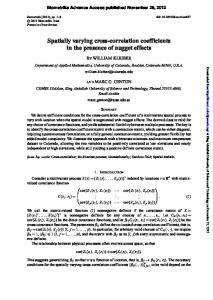
3.3. Sample size requirements For the 1694 correlation matrices generated, the resulting absolute values of g ranged from 0 to .56 and the resulting values of s2 ranged from .0004 to 1.45. From these matrices, we selected the 1226 matrices that produced absolute g values above 0 and at or below.30 as we suspect that these are the values most likely to be encountered in applied research.

172 Razia Azen and Daniel A. Sass

Figure 2. Sample estimates (s^ 2 ) of population variance (s2, shown as horizontal line) averaged over 5000 replications.

For each of these 1226 matrices, the value of s and the minimum sample size needed to achieve 80% power were computed. The results are presented in Figure 6, where it can be seen that smaller g values tend to be associated with a wider range of s values and that even with reasonable g-values (e.g. .05) one may require well over 200–300 observations to Table 3. Null case: estimates of Type I error rates, or percentage of null hypothesis (H0: g ¼ 0) rejections over 5000 replications, by sample size Matrix A: g ¼ 0

Sample size

H0 rejection rate

95% CI coverage rate

50 100 150 200 250 300 400 500 600 700 800 900 1000

5.0 5.5 5.7 5.1 5.2 5.5 5.0 4.8 5.0 5.1 5.1 5.2 5.3

95.0 94.5 94.3 94.9 94.8 94.5 95.0 95.2 95.0 94.9 94.9 94.8 94.7

Comparing squared multiple correlations

173

Table 4. Non-null cases: percentage of null hypothesis (H0: g ¼ 0) rejections and percentage of 95% confidence intervals that contained g over 5000 replications, by sample size Sample size

H0 rejection rate

95% CI coverage rate

B: g ¼ .05

50 100 250 500 1000

5.3 20.7 72.1 96.8 100.0

90.2 91.8 93.6 94.4 94.9

C: g ¼ .10

50 100 250 500 1000

18.6 32.5 63.6 90.1 99.6

93.0 94.5 94.5 95.4 95.5

D: g ¼ .15

50 100 250 500 1000

24.7 44.4 81.6 98.0 99.9

93.3 94.2 95.0 95.5 95.0

E: g ¼ .20

50 100 250 500 1000

55.7 91.7 100.0 100.0 100.0

90.9 93.2 94.3 95.1 95.0

F: g ¼ .25

50 100 250 500 1000

56.7 84.0 99.7 100.0 100.0

93.0 93.8 94.8 94.7 95.2

G: g ¼ .30

50 100 250 500 1000

84.2 98.7 100.0 100.0 100.0

92.8 93.6 94.4 95.1 95.0

Matrix

Note. For all matrices, the rejection rate represents power and the expected coverage rate was 95%.

achieve adequate power. In addition, it is not at all unusual for small g values (under .05) to require very large sample sizes (often well above 500) to achieve adequate power, and for very small g values (of about .01) it appears that minimum sample sizes greater than 1000 are the rule rather than the exception. To further illustrate the effect that the value of s has on the power and required sample size for the procedure, consider the four matrices presented in Table 5. Note that while all matrices have the same g-value (i.e. g ¼ .04), small changes in the matrix produce different s values that, in-turn, lead to different g/s ratios and very different minimum sample size requirements. For example, matrix I in Table 5 produces s ¼ .27, g/s ¼ .16, and the minimum sample size required to achieve 80% power is just under

174 Razia Azen and Daniel A. Sass

Figure 3. Coverage rates of 95% confidence intervals over 5000 replications, by sample size.

300. A change in only one element of the matrix (the correlation between X2 and X3) results in s ¼ .33, a g/s ratio of .14 and a minimum sample size requirement that is now over 400 (matrix II). Further, matrix IV results in s ¼ .57, a g/s ratio of .08 and a minimum sample size requirement of over 1300. A programme that provides the values of g and s and computes the expected minimum sample size requirements, given a userspecified population correlation matrix, is available from the authors at http://www. uwm.edu/~azen/r2infmacro.html.

4. Discussion In general, Olkin and Finn’s (1995) sample size recommendations for confidence intervals seem to be supported by the results of this simulation study. For sample sizes greater than 200, it appears that coverage rates are reasonably satisfied by the asymptotic procedure for comparing squared multiple correlations from two non-nested models. However, for hypothesis testing purposes, these sample size guidelines are often inadequate. Regarding statistical power, it is not entirely possible to make a general statement as to sample size requirements for this procedure. For example, Table 4 (and Figures 4 and 5) show that for a given sample size (e.g. 250) some matrices or combinations of parameters achieve adequate power levels (e.g. matrix D obtains power of 81.6% with n ¼ 250) while other matrices do not (e.g. matrix C obtains power of 63.6% with n ¼ 250). Therefore, although the 95% confidence interval performs adequately

Comparing squared multiple correlations

175

Figure 4. Power (null hypothesis rejection) rates over 5000 replications, by sample size.

with samples of 250 in almost all cases, power may be less than adequate in many cases (even with the same sample size). The reason for this is that while the confidence interval may contain the parameter (g) with probability close to 95%, the same interval also contains zero with higher than desired probability leading to too few null hypothesis rejections. In fact (everything else being equal), sample size requirements for

Figure 5. Observed (points) and expected (lines) power rates over 5000 replications, by sample size.

176 Razia Azen and Daniel A. Sass

Figure 6. The relationship between absolute value of g, s and the minimum sample size required to obtain 80% power for 1226 matrices with 0 , jgj # 0.30.

a given power rate vary inversely with the absolute value of the ratio g/s, but for a given value of g the standard deviation s is difficult to predict and thus power is not readily predictable either. This point is further illustrated in Table 5 and Figure 6. Therefore, researchers should be aware that while 200–300 observations may provide adequate coverage rates (i.e. confidence intervals), for hypothesis testing purposes the effect (g) is not sufficient to determine the sample size required for an acceptably powerful test; instead, the g/s ratio needs to be estimated. Researchers who have some idea of the g value they are expecting can use Figure 6 for guidelines as to the range of sample sizes that may be required for their study or obtain a more precise estimate using a programme available from the authors. This study has implications for researchers wishing to compare two non-nested models by testing differences between their R2 values. Dominance Analysis (Azen & Budescu, 2003; Budescu, 1993), for example, is based on such comparisons, and the findings presented here will inform the development of statistical tests for quantitative Dominance Analysis results that have not yet been investigated and evaluated. The main finding of this study is that sample size considerations vary widely, especially for small values of g, and the power of the procedure in these cases may be inadequate even with traditionally reasonable sample sizes.

Comparing squared multiple correlations

177

Table 5. Minimum sample size required to achieve 80% power for four population correlation matrices with g ¼ .04 Matrix I

II

III

IV

Y X1 X2 X3

Y 1.0 .7 .3 .3

Y X1 X2 X3

1.0 .7 .3 .3

Y X1 X2 X3

1.0 .3 .3 .1

Y X1 X2 X3

1.0 .3 .3 .3

X1

X2

X3

1.0 .1 .3

1.0 .5

1.0

1.0 .1 .3

1.0 .3 .1

1.0 .1 .5

1.0 .1

1.0 .3

1.0 .1

g

s

r2

r2(Y·X1X2)

g/s

Min n

.0445

.2733

.54

.54

.16

296

.0445

.3288

.55

.54

.14

428

.0435

.3846

.14

.14

.11

614

.0436

.5657

.19

.16

.08

1320

1.0

1.0

1.0

While this study is limited in that it did not examine all possible correlation matrices that may occur in practice, there is no particular reason to expect that these results will not generalize to most practical situations. In addition, this study was concerned only with testing the difference between relatively simple models that each consisted of two predictors (i.e. X1 and X2 compared to X1 and X3) and the results have not been extended to a comparison of models with three or more predictors. Procedurally, however, including additional predictors is a relatively straightforward extension of the method discussed here (i.e. the a vector discussed in the methods section would simply be defined to include higher-order models), so adding predictors will not affect the results of the model comparisons presented here. Finally, multivariate normal data and methods appropriate for such data were used in this paper, but these methods may not be optimal for non-normal data (e.g. Steiger & Browne, 1984; Steiger & Hakstian, 1982). In conclusion, the asymptotic method developed by Olkin and his colleagues can be used to construct confidence intervals with sample sizes over 200–300. However, the power of testing null hypotheses of the form g ¼ 0 is quite low unless the g/s ratio is rather large, and the value of s appears to be quite variable especially for small (but practical) values of g. R2 differences that are greater than approximately .15 can be detected with adequate power using reasonable sample sizes, but lower differences require very large (and possibly unfeasible) sample sizes. Finally, because the value of s is quite variable and involves all elements of the (predictors and response) correlation matrix, researchers cannot assume that a reasonable value of g (that appears to represent a practically significant effect) will necessarily yield

178 Razia Azen and Daniel A. Sass

a sizable g/s ratio that can be readily detected statistically with null hypothesis testing. Further research is clearly needed for a more powerful test of small to medium g values (i.e. g , .10), as these are most likely to occur in applied research. In the meantime, this study provides valuable insights into the performance of the asymptotic method and its sample size requirements.

References Alf, E. F., & Graf, R. G. (1999). Asymptotic confidence limits for the difference between two squared multiple correlations: A simplified approach. Psychological Methods, 4, 70–75. Algina, J., & Keselman, H. J. (1999). Comparing squared multiple correlation coefficients: An examination of a confidence interval and a test of significance. Psychological Methods, 4, 76–83. Azen, R., & Budescu, D. V. (2003). The dominance analysis approach for comparing predictors in multiple regression. Psychological Methods, 8, 129–148. Azen, R., Sass, D. A., & Budescu, D. V. (2004). Predictor importance in multiple regression: Inferential methods for Dominance Analysis. Poster presented at the Annual Convention of the American Psychological Association, Honolulu, Hawaii. Bradley, J. V. (1978). Robustness? British Journal of Mathematical and Statistical Psychology, 31, 144–152. Budescu, D. V. (1993). Dominance analysis: A new approach to the problem of relative importance of predictors in multiple regression. Psychological Bulletin, 114, 542–551. Budescu, D. V., & Azen, R. (2004). Beyond global measures of relative importance: Some insights from dominance analysis. Organizational Research Methods, 7, 341–350. Cohen, J. (1988). Statistical power analysis for the behavioral sciences (2nd ed.). Hillsdale, NJ: Erlbaum. Graf, R. G., & Alf, E. F. (1999). Correlations redux: Asymptotic confidence limits for partial and squared multiple correlations. Applied Psychological Measurement, 23, 116–119. Hedges, L. V., & Olkin, I. (1981). The asymptotic distribution of commonality components. Psychometrika, 46, 331–336. Hedges, L. V., & Olkin, I. (1983). Joint distributions of some indices based on correlation coefficients. In S. Karlin, L. A. Goodman, & F. Amemiya (Eds.), Studies in econometrics, time series, and multivariate analysis (pp. 437–454). New York: Academic Press. Johnson, J. W., & LeBreton, J. M. (2004). History and use of relative importance indices in organizational research. Organizational Research Methods, 7, 238–257. Olkin, I., & Finn, J. D. (1995). Correlations redux. Psychological Bulletin, 118, 155–164. Olkin, I., & Siotani, M. (1976). Asymptotic distribution of functions of a correlation matrix. In S. Ikeda (Ed.), Essays in probability and statistics (pp. 235–251). Tokyo: Shinko Tsusho. Pedhazur, E. J. (1997). Multiple regression in behavioral research (3rd ed.). Orlando, FL: Harcourt Brace. Rowell, R. K. (1996). Partitioning predicted variance into constituent parts: How to conduct regression commonality analysis. In B. Thompson (Ed.), Advances in social science methodology (Vol. 4. pp. 33–43). Greenwich, CT: JAI Press. Steiger, J. H., & Browne, M. W. (1984). The comparison of interdependent correlations between optimal linear composites. Psychometrika, 49, 11–21. Steiger, J. H., & Hakstian, A. R. (1982). The asymptotic distribution of elements of a correlation matrix: Theory and application. British Journal of Mathematical and Statistical Psychology, 35, 208–215. Received 14 April 2006; revised version received 20 November 2006