Comparing two formulations of skew distributions with special

arXiv:1402.5431v1 [math.ST] 21 Feb 2014

Comparing two formulations of skew distributions with special reference to model-based clustering Adelchi Azzalini∗ Ryan P. Browne† Marc G. Genton‡ Paul D. McNicholas†

Abstract Multivariate skew distributions continue to gain popularity as effective tools in data analysis for a wide variety of data types. They also feature in several modern computational statistics techniques, including model-based clustering approaches. Two well-known formulations of skew distributions have been used extensively within the model-based clustering literature over the past few years. We investigate the properties of these formulations and, in doing so, we refute various claims that have been made about these formulations of late. Our position as to the inaccuracy of these claims is supported by theoretical arguments as well as real data examples.

1

Background and Motivation

In the last 10–15 years, much work in the statistical literature has been dedicated to the development of flexible parametric classes of distributions, with special interest in the multivariate case where the set of alternatives to the normal distribution is not as wide as in the univariate case. When the domain of interest is the d-dimensional Euclidean space, the class of elliptical distributions is the more studied alternative to the normal family, of which it represents a superset. However, because the elliptical class imposes stringent symmetry conditions, which must hold simultaneously for all components of the distribution, this calls for the development of more flexible families to more closely meet the data behaviour in a number of real cases. When one moves away from the symmetry of the multivariate normal or the elliptical distributions, the feature that arises more easily is skewness, and this explains the widespread use of the prefix ‘skew’ which recurs almost constantly in this context. The specific, but already quite broad, stream of literature we are referring to is commonly identified by terms like ‘skew-symmetric’, ‘skew-elliptical’ and similar ones. A recent extensive account is provided by Azzalini and Capitanio (2014). This activity has generated an enormous number of formulations, sometimes arising with the same motivation and target, or nearly so. A natural question in these cases is which of the competing alternatives is preferable, either universally or for some given purpose. To be more specific, start by considering the multivariate skew-normal (SN) distribution proposed by Azzalini and Dalla Valle (1996), examined further by Azzalini and Capitanio (1999) and by much subsequent work. Note that, although the latter paper adopts a different parameterization of the earlier one, the set of distributions that they encompass is the same; we shall denote this construction as the ‘classical skew-normal’. Another form of skew-normal distribution has been studied by Sahu, Dey, and Branco (2003), which we shall refer to as the ‘SDB skew-normal’. The classical and the SDB set of distributions coincide only for dimension d = 1; otherwise, the two sets differ and not simply because of different parameterizations. For d > 1, the question then arises about whether ∗ Department

of Statistical Science, University of Padua, 35121 Padova, Italy. of Mathematics & Statistics, University of Guelph, Guelph, Ontario, Canada. ‡ CEMSE Division, King Abdullah University of Science and Technology, Thuwal, Saudi Arabia. † Department

1

there is some relevant difference between the two formulations from the viewpoint of suitability for statistical work, both on the side of formal properties and on the side of practical work. The above-described situation carries on with the broader formulations that arise when in the underlying parent distribution the normal family is replaced by the wider elliptical class, leading to the so-called skewelliptical distributions. A special case that has received much attention is the skew-t family, which was formulated by Branco and Dey (2001) and examined in detail by Azzalini and Capitanio (2003). Again, this ‘classical’ skew-t has a counterpart given by another skew-t considered by Sahu et al. (2003), and the same questions as above hold. For both forms of skew-t distribution, a major reason for their appeal is represented by the great flexibility of the density shape, which arises because we can regulate the tail weight via the degrees of freedom, like with the traditional Student’s t distribution, as well as the slant of the distribution via a d-vector asymmetry parameter. A substantial fraction of the work in this direction has been generated in the context of modelbased clustering, which involves introducing a mixture density of the form f (x) =

G X

πg f0 (x; θg ),

x ∈ Rd ,

(1)

g=1

PG where πg > 0, with g πg = 1, is the mixing proportion for the gth component, f0 is a parametric family of distributions and θg is the parameter set of the gth mixture component within this family. The additional flexibility of the skew-t distribution if used in the role of f0 , compared to the multivariate normal and Student’s t, can diminish the number of components G required to fit the data adequately when the data points are grouped in non-elliptical clusters, leading to a more easily parsimonious and a possibly more interpretable outcome. There is an additional reason for paying special attention to this portion of the model-based clustering literature. In connection with the use of the above-recalled distributions, some views have been formulated quite recently which we believe to be unjustified and inaccurate, with effects that might potentially have unintended impact beyond the model-based clustering community. We are referring to the formulation of Lee and McLachlan (2014), to which for brevity we shall indicate as LM2012 because the paper appeared online in 2012. The authors have subsequently adopted the same framework in other publications (e.g., Lee and McLachlan, 2013b,c). The overall aim of the present paper is to present a detailed comparison of the two formulations, classical and SDB, as for their formal properties and suitability in applied work, and to discuss the view formulated by Lee and McLachlan in the publications mentioned above.

2 2.1

Skew-normal and Skew-t Distributions Two skew-normal formulations

Because of their role as the basic constituent for more elaborate formulations, we start by discussing the two forms of skew-normal distributions. The density and the distribution function of a Nd (0, Σ) variable are denoted ϕd (·; Σ) and Φd (·; Σ), respectively; the N (0, 1) distribution function is denoted Φ(·). The classical skew-normal density function is fc (x) = 2 ϕd (x − ξ; Ω) Φ{α> ω −1 (x − ξ)},

x ∈ Rd ,

(2)

with parameter set (ξ, Ω, α). Here ξ is a d-dimensional location parameter, Ω is a symmetric positive definite d × d matrix, playing the role of scale parameter, α is a d-dimensional slant parameter and ω is a diagonal matrix formed by the square roots of the diagonal elements of Ω.

2

Various stochastic representations exist for (2). One is as follows: if     ¯ δ X0 Ω ∗ ∗ ∼ Nd+1 (0, Ω ), Ω = X1 δ> 1 where Ω∗ is a correlation matrix, then Yc = ξ + ω(X0 |X1 > 0)

(3)

¯ and α = (1 − δ > Ω ¯ −1 δ)−1/2 Ω ¯ −1 δ. Another stochastic representation is has distribution (2) with Ω = ω Ωω the following: if δ is a d-vector with elements in (−1, 1), (2) is the density function of n o Yc = ξ + ω [Id − diag(δ)2 ]1/2 V0 + δ|V1 | , (4) where V0 and V1 are independent normal variates of dimension d and 1, respectively, with 0 mean value, unit variances and cor(V0 ) is suitably related to α and Ω. The moment generating function of (2) is Mc (t) = 2 exp(t> ξ + t> Ωt/2)Φ(t> ωδ), from which we obtain the mean value and the variance matrix p var(Yc ) = Ω − (2/π) ωδ δ > ω, E(Yc ) = ξ + 2/π ωδ, ¯ −1/2 Ωα. ¯ where δ = (1 + α> Ωα) A more detailed exposition of the above facts is presented in Chapter 5 of Azzalini and Capitanio (2014), together with additional properties of the distribution. For the SDB skew-normal, we adopt a very minor change from the symbols of Sahu et al. (2003), but retain the same parameterization. Given real values λ1 , . . . , λd , let λ = (λ1 , . . . , λd )> ,

Λ = diag(λ)

and write the SDB density as fs (x) = 2d ϕd (x − ξ; ∆ + Λ2 ) Φd {Λ(∆ + Λ2 )−1 (x − ξ); Id − Λ(∆ + Λ2 )−1 Λ},

(5)

where ∆ is a symmetric positive-definite matrix. This density is associated with the following stochastic representation. For independent variables ε ∼ Nd (ξ, ∆) and Z ∼ Nd (0, Id ), consider the transformation Ys = Λ(Z|Z > 0) + ε,

(6)

where Z > 0 means that the inequality is satisfied component-wise; then Ys has density (5). The moment generating function of fs is  Y d Ms (t) = 2d exp t> ξ + t> (∆ + Λ2 )t/2 Φ(λj tj ),

(7)

j=1

which by differentiation leads to E(Ys ) = ξ +

p

2/π λ ,

var(Ys ) = ∆ + (1 − 2/π)Λ2 .

(8)

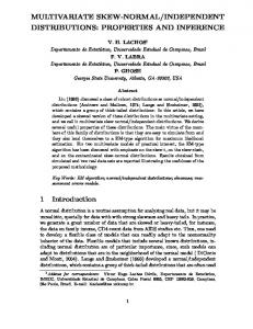
To obtain a first perception of the density shape of the two distributions, we produce plots which are the direct analogue of Figures 4 and 5 of Azzalini and Dalla Valle (1996) originally used to illustrate the classical skew-normal. The left panel of our Figure 1, which matches their Figure 4, displays a scatter plot of the weight (Wt, in kg) and the height (Ht, in cm) of 202 athletes examined at the Australian Institute of Sport (AIS), with the classical SN fit superimposed; in addition, we also plot the corresponding fit of the SDB 3

40

160

50

170

60

LBM 70

Ht 180

80

190

90

200

100

210

density. The right panel of Figure 1 displays a similar plot for the lean body mass (lbm) and body mass index (bmi) of the same athletes. The contour level curves of the classical and the SDB densities turn out to be very similar. In the left panel, the two sets of contour curves are virtually identical; in the right panel, the modes are somewhat displaced and the SDB curves have more spiky corners than the classical density, but again the densities are otherwise very similar. The AIS data, which comprise several other variables, have been used extensively for illustrative purposes in the subsequent literature, effectively becoming a sort of standard benchmark; therefore, we shall employ them again in the coming sections.

150

classical SDB 40

60

80 Wt

100

classical SDB

120

20

25 BMI

30

35

Figure 1: AIS data: scatter plot of (Wt, Ht) in the left panel and of (BMI, LBM) in the right panel, with superimposed fitted distributions using the classical and the SDB skew-normal families. A qualitative comparison of the formal properties of the two distributions lends several annotations. Some of these have already been presented by Sahu et al. (2003), but they are included here for completeness. 1. Distributions (2) and (5) are regulated by the parameter sets (ξ, Ω, α) and (ξ, ∆, λ). The two sets match as for nature and dimension of the three components; the number of individual parameter values is 2d + d(d + 1)/2 in both cases. 2. As remarked by Sahu et al. (2003), the two distributions coincide only for d = 1. We underline that for d > 1 neither one of the two families is a subset of the other. To see this fact, consider matching the arguments of exp(·) in the moment generating functions by choosing a common ξ and Ω = ∆ + Λ2 . The final factors of Mc and Ms , however, cannot match if d > 1, because in Ms there is the product of several Φ terms, while Mc has only one such term. 3. If d is not small, computation of fs becomes cumbersome because of the Φd factor. Computational techniques, such as those described by Genz and Bretz (2009), facilitate handling this problem, but the burden involved increases rapidly with d. For example, LM2012 only consider examples with d ≤ 4. 4. The classical skew-normal family is closed under affine transformations, while the same fact does not hold for the SDB family. The first part of this statement is widely documented in the above-quoted literature. For the second part, consider a linear transformation Xs = A Ys for some non-singular matrix A, and notice that this is equivalent to replacing Λ in (6) by a non-diagonal matrix. 4

5. Another remark of Sahu et al. (2003) is that fs can allow for d independent skew-normal components, when ∆ is diagonal, while fc can factorize only as a product where at most one factor is skew-normal with non-vanishing slant parameter. 6. Stochastic representations (3) and (6) involve 1 and d latent variables, respectively. The latter one seems to fit less easily in an applied setting, because it requires that for each observed component there is a matching latent component, while the classical construction can more easily be incorporated in the logical frame describing a real phenomenon subject to selective sampling based on one latent variable. 7. For the classical skew-normal, the expressions of higher order cumulants and Mardia’s coefficients of multivariate skewness and kurtosis are given in Appendix A.2 of Azzalini and Capitanio (1999). The range of skewness is [0, g1∗ ) where g1∗ = 2(4 − π)2 /(π − 2)3 ≈ 0.9905658; the range of excess kurtosis is [0, g2∗ ), where g2∗ = 8(π − 3)/(π − 2)2 ≈ 0.869177. For the SDB form, expressions of Mardia’s coefficients are given in an appendix of the present paper. Numerical maximization of these expressions when d = 2 leads to the range [0, 1.98113) and [0, 1.738354), whose maximal values appear to coincide numerically with 2 g1∗ and 2 g2∗ , respectively. 8. For the classical skew-normal, the distribution of quadratic forms can be obtained from the similar case under normality; for instance, we can state that (Yc − ξ)> Ω−1 (Yc − ξ) ∼ χ2d . This fact is useful, among other things, for building QQ-plots of model adequacy. No similar result is known to hold for the SDB form. Because the indication emerging from these remarks is not completely in favour of either of the two formulations, the choice is a matter of emphasis on one or another aspect, depending on the specific problem of interest or even individual preference. However, for the Mardia’s coefficients, we notice that the wider range of the SDB formulation is not a crucial aspect, because for both fc and fs these coefficients have a very small range anyway, and the limitations are to be overcome by the introduction of the corresponding skew-t families. A possibly more important point is the factorization issue of Remark 5, if this aspect is relevant for the specific problem under consideration. On the other hand, the lack of closure under affine transformations can be a non-negligible limitation in a range of problems. Sahu et al. (2003, p. 132) observe that the fs distribution could be extended to the case of non-diagonal matrices. This route does not seem to have been developed, presumably because it has been subsumed in the even more general ‘closed skew-normal’ formulation of Gupta et al. (2004) and Gonz´ alezFar´ıas et al. (2004). The adoption of the closed skew-normal distribution would also have the advantage of replacing the factor Φd in (5) by one of type Φm , where we can take m < d. Also the interpretability issue of Remark 6 can be of relevance if one is concerned with qualitative and subject-matter plausability of the formulation. An additional aspect of these densities is illustrated graphically. Figure 2 refers to bivariate distributions having parameters       0 1 1/2 30 ξ= , Ω=∆= , α=λ= 0 1/2 1 50 with (Ω, α) employed for the clasical SN on left-side plot and (∆, λ) employed for the SDB density on the right-hand plot. The slant parameters α and λ, respectively, are sufficiently large to indicate the limit behaviour of the densities when these parameters diverge. In the first case, the support of the density approaches the half-plane {(x, y) : α1 ω1−1 x + α2 ω2−1 y ≥ 0}, with ω1 = ω2 = 1 in this case; in the second diagram, the support reduces to one of the quadrants, identified by the signs of the λ components. A well-known issue with the likelihood function associated to the classical SN distribution is the systematic presence of a stationarity point of the profile log-likelihood at α = 0. This aspect is linked to another one, that is, singularity of the information matrix at α = 0. Given the ensuing complication to the inferential 5

120

3

80

100

2

60

y

1 y

20

40

0

0

−1 −2

−1

0

1

2

3

0

x

10

20

30

40

50

60

70

x

Figure 2: Contour level plots of the classical and SDB density where the slant parameters diverge. process when the MLE estimate α ˆ is close to 0, a natural question is whether the SDB version is free of this problem. A simple answer is possible in the special case when ∆ is diagonal. Factorization of the fs density, underlined in Remark 5, translates into factorization of the likelihood function into the product of d likelihoods, each of univariate SN type with slant parameter equal to 0. Hence the stationarity problem and its implication persist also with the SDB density. When ∆ is not diagonal, the question becomes algebraically more intricate. Because a detailed analysis of the question would involve a project on its own, we have confined ourselves to some numerical explorations, which have confirmed the qualitative indications of the case with a diagonal ∆. The end conclusion is that, also on this front, the two formulations behave in a qualitatively analogous way.

2.2

Corresponding skew-t distributions

Each of the two skew-normal families discussed above leads to a matching form of skew-t family. For the classical case, this can be obtained by replacing the assumption of joint normality of (X0 , X1 ) in (3) by one of (d + 1)-dimensional Student’s t distribution; this has been formulated by Branco and Dey (2001) and examined further by Azzalini and Capitanio (2003). The SDB skew-t has been obtained by Sahu et al. (2003) assuming that (Z, ε) entering (6) is a (2d)-dimensional Student’s t. In both cases, the resulting density is similar in structure to the skew-normal case, with the ϕd term replaced by a d-dimensional t density on ν degrees of freedom, but the skewing factor is different: for the classical version, it is given by the distribution function of a univariate t on ν + d degrees of freedom; for the SDB version, the t distribution function is d-dimensional. The shape of these densities is qualitatively similar to their corresponding SN density, but with more elongated tails; therefore, we do not present specific plots. The classical skew-t can also be generated via a construction that closely resembles that of the regular Student’s t, as follows: given a classical skew-normal variate Zc with location ξ = 0 and an independent

6

V ∼ χ2ν /ν, the variable

√ Xc = ξ + Zc / V

has the same distribution as the classical skew-t described above. We are not aware of a similar type of representation for the SDB skew-t. Both types of skew-t distribution involve only one extra parameter, ν, compared to the skew-normal. However, this is sufficient to widen considerably the range of feasible values of the coefficients of skewness and kurtosis, both marginally for each component and for the global Mardia’s coefficients. It also allows to regulate separately skewness and kurtosis, which are instead interlinked in the skew-normal distribution. We refer the reader to the original sources for more details on this point. This increased flexibility in the skew-t family, in either version, makes it especially appealing for practical data fitting; we shall explore this aspect in the next section. As anticipated earlier, we now discuss some of the statements by Lee and McLachlan, in the paper denoted earlier LM2012 and related ones, with respect to the formal properties established above; an analogous discussion concerning the more applied side is deferred to the subsequent sections. In these expositions the skew-normal and skew-t distributions which we refer to as classical are named ‘restricted’ and those that we refer to as SDB are named ‘unrestricted’, under the incorrect presumption that the SDB variants constitute a more general family than the classical ones. To be specific, the opening sentence of Section 2.2 of LM2012 states that “The unrestricted multivariate skew-normal (uMSN) distribution can be viewed as a simple extension of the rMSN distribution in which the univariate latent variable U0 is replaced by a multivariate analogue, that is, U0 ”, where rMSN stands for restricted multivariate skew-normal and their U0 is V1 in (4). The same conviction is replicated near the end of the same section. Not only does the adopted terminology, restricted vs. unrestricted, convey a message of broader generality in the second case, but this is also explicit in the use of the term ‘extension’, which is inappropriate because we have seen earlier that neither one of the two families is a subset of the other for d > 1. Notice that no such claim of wider generality had been made by Sahu et al. (2003). Furthermore, in the discussion of the classical skew-t distribution near the end of Section 3 of LM2012, the authors state that “the form of skewness is limited in these characterizations. In Sect. 5 we study an extension of their approach to the more general form of skew t-density as proposed by Sahu et al. (2003).” This claim of limited form of skewness is completely unsupported; no expressions of any measure of skewness is even reported. As a matter of fact, the opposite is true: the range of skewness for the classical skew-t distribution is unlimited both marginally, when measured by the usual coefficient γ1 , and globally, when measured by Mardia’s coefficient γ1,d . To see this fact in the univariate case, which coincides with the behaviour of univariate components in a multivariate skew-t distribution, consider the expression of γ1 on p. 382 of Azzalini and Capitanio (2003) and let ν → 3; for the Mardia’s coefficient, see (6.31) on p. 178 of Azzalini and Capitanio (2014).

3 3.1

Model-based Clustering with Skew-t Distributions Preliminary remarks

The above-recalled distributions have been employed not only in a range of numerical illustrations of theoretical papers but also in various genuine applied problems and as ingredients for methodological developments. For the purpose of data-fitting, the skew-t distributions, in either form, have more potential because of the additional tail-weight parameter. Although in both variant forms there is a single parameter regulating the tail behaviour, this has proved to work effectively in a large number of cases. It is not our purpose here to present a general review of all this work, which would take considerable space, but at least we like to mention the paper of Azzalini and Genton (2008) because it provides numerical illustrations in several diverse areas, with favourable results in all cases. Taking into account that the SDB 7

formulation seems to have been employed relatively more often in the context of mixture distributions of type (1), we focus our attention in this direction by focusing on model-based clustering applications. Moreover, model-based clustering represents the context where LM2012 and related publications are placed. Again, some of the statements made therein have provided further motivation for writing the present note. Similarly to the questionable statements on the theoretical aspects discussed in Section 2, LM2012 contains claims like “the superiority of FM-uMST model is evident” (end of Section 6.1) and “the extra-flexibility offered by the more general FM-uMST model” (end of Section 6.2). These comments refer to two specific cases, but are taken as the basis for the general statement “Examples on several real datasets shows [sic] that the unrestricted model is capable of achieving better clustering than the restricted model” (Section 8). Besides these specific passages, the general tone of the paper conveys a message of overall superiority of the SDB formulation, and we believe this is unjustified. It is the purpose of the remaining part of this section to explore in a more systematic and fairer way the performance of the two forms of skew-t distributions in clustering applications. An important aspect in these comparisons is the potential bias due to selective reporting. To avoid the perception of bias that can arise from selection of a subset of variables from a data set like the AIS data, we examine all possible pairs and triplets of variables in our real data illustrations (Section 3.5). Note that there is much other work on model-based clustering using skewed distributions. Some of this work is based on the formulations already discussed in this paper (e.g., Pyne et al., 2009; Lin, 2009, 2010; Lin et al., 2013; Vrbik and McNicholas, 2012, 2014). However, there is also a substantial amount of work on model-based clustering using other skewed distributions (e.g., Karlis and Santourian, 2009; Ho et al., 2012; Murray et al., 2013; McNicholas et al., 2013; Browne and McNicholas, 2013; Franczak et al., 2014). In the analyses given herein, we focus only on comparison of the two skew-t formulations that are the subject of the present paper.

3.2

Performance assessment

Although the illustrations herein are conducted as genuine cluster analyses, i.e., no knowledge of labels is assumed, the true labels are known; accordingly, we can asses the classification performance of the fitted models. The adjusted Rand index (ARI; Hubert and Arabie, 1985), which is a corrected version of the Rand index (Rand, 1971), is used for this purpose. The ARI takes a value of one when there is perfect agreement between two classes, or two partitions in general, and its expected value is zero under random classification. Negative values are also possible and indicate classification that is worse than would be expected by guessing.

3.3

Implementation

We implement the classical and SDB skew-t mixture models in the R software (R Core Team, 2013), and our implementations will be made available as a function within the mixture package. Starting values were obtained using k-means clustering and for each data set, the same starting values were used for each approach.

3.4

Simulated data

A two-dimensional data set is simulated to illustrate a difficult clustering problem, where one cluster lies within the other (Figure 3). One component (black in Figure 3) is generated from a SDB skew-t distribution and the other (red in Figure 3) from a classical skew-t distribution. Each component contains 1,000 observations. Mixtures of classical and SDB skew-t distributions, respectively, are fitted to these simulated data in a model-based clustering framework with G = 2 components. The results (Figure 4 and Table 1) show that both classical and SDB skew-t mixtures give very good classification performance, with the classical

8

25 20 15 10 x2 5 0 -5 -10

-10

-5

0

5

10

15

20

x1

Figure 3: Scatter plot illustrating the simulated data, coloured by component. skew-t mixture giving slightly better classification performance (ARI=0.781) than the SDB skew-t mixture (ARI=0.774).

20 15 10 -10

-5

0

5

x2 -10

-5

0

5

x2

10

15

20

25

SDB Skew-t

25

Classical Skew-t

-10

-5

0

5

10

15

20

-10

x1

-5

0

5

10

15

20

x1

Figure 4: Scatter plot of the predicted classifications for the classical (left) and SDB (right) skew-t mixtures applied to the simulated data, where colour represents predicted classifications.

3.5

Crabs data

Campbell and Mahon (1974) report data on five biological measurements of 200 crabs of genus leptograpus. The data were collected in Fremantle, Western Australia, and comprise 50 male and 50 female crabs for each 9

Table 1: Cross-tabulations of true (A,B) and predicted (1,2) group memberships for the classical and SDB skew-t mixtures, respectively, for the simulated data. Classical A B

1 952 68

SDB 2 48 932

1 942 62

2 58 938

14 6

8

10

12

RW

16

18

20

of two species. These data are available in the MASS package for R, which contains data sets from Venables and Ripley (1999). We focus on these data because they have been used throughout the model-based clustering literature to illustrate the performance of various methods. First, we focus on two of the five variables, i.e., frontal lobe size (FL) and rear width (RW), both measured in millimetres. Based on these variables, it should be possible to recover gender within a clustering framework (cf. Figure 5). Mixtures of classical and SDB skew-t distributions, respectively, are fitted to the crabs data in a model-based clustering framework with G = 2 components. The results (Table 2 and Figure 6) show

10

15

20

FL

Figure 5: Scatter plot illustrating two variables (FL, RW) from the crabs data, coloured by gender. that the classical skew-t mixture model gives good classification performance with only 30 misclassifications, corresponding to an ARI of 0.487. The SDB skew-t mixture model, however, gives very poor classification, producing results only slightly better than would be expected under random classification (ARI=0.074), with 72 of the 200 crabs misclassified. Table 2: Cross-tabulations of true and predicted group memberships for the classical and SDB skew-t mixtures, respectively, for the crabs data. Classical Male Female

1 83 13

SDB 2 17 87

1 83 55

10

2 17 45

18 16 14 6

8

10

12

RW

14 6

8

10

12

RW

16

18

20

SBD Skew-t

20

Classical Skew-t

10

15

20

10

FL

15

20

FL

Figure 6: Scatter plot illustrating predicted classifications for the classical (left) and SDB (right) skew-t models applied to the crabs data, where colour represents predicted classifications. We previously remarked (Section 3.1) that presenting results based on a subset of variables in a data set may incur bias or at least a perception thereof. Accordingly, a more comprehensive analysis is also undertaken, wherein mixtures of classical and SDB skew-t distributions, respectively, are applied to all possible pairs and triplets of variables of the crabs data within a model-based clustering framework. Note that we take gender as the true class, which is consistent with the analysis of Peel and McLachlan (2000) who considered two variables of the crabs data. The results of these analysis are presented in Figure 7, which gives the ARI values for the analyses with the classical and SDB skew-t distributions, respectively, for all pairs and triplets. It is visible that in most cases the points are close to the identity line; hence indicating no advantage of either one formulation over the other. The only point departing significantly from this pattern is based on a pair and indicates a preference for the classical skew-t distribution; this point corresponds to the pair (FL, RW) examined earlier. The group of points near the bottom-left corner arises because some of the variables do not exhibit any discriminatory capability due largely to their very high correlation.

11

1.0 0.8 0.6 0.4

Classical Skew-t

0.2 0.0 0.0

0.2

0.4

0.6

0.8

1.0

SDB Skew-t

Figure 7: ARI values from analyses of all pairs (black circles) and triplets (triangles) of variables in the crabs data using classical and SDB skew-t distributions, respectively.

3.6

AIS data

0.6 0.4 0.0

0.2

Classical Skew-t

0.8

1.0

We also consider the AIS data, which provide 11 biomedical and anthropometric measurements and two categorial variables, i.e., gender and sport, for each of 202 Australian athletes. Some of these variables have already appeared herein (Figure 1). The reason for considering these data is that they have been extensively used for illustrative purposes in the literature on skew-symmetric distributions. We proceed similarly to the crabs data, by considering all possible pairs and triplets of the continuous measurements to build clusters of the data points. To compute the ARI index, we again take gender as the reference classifying variable. The results are summarized in Figure 8, which is constructed in an analogous fashion to Figure 7. The message clearly delivered by the new figure is that of an overall equivalence between the two families of distributions in this comparative exercise.

0.0

0.2

0.4

0.6

0.8

1.0

SDB Skew-t

Figure 8: ARI values from analyses of all pairs (black circles) and triplets (triangles) of variables in the AIS data using classical and SDB skew-t distributions, respectively.

12

3.7

Comments

1.0 0.8 0.6 0.0

0.2

0.4

Classical Skew-t

0.6 0.4 0.0

0.2

Classical Skew-t

0.8

1.0

One may argue that our results for the analysis of the crabs and AIS data sets are merely an artifact of our software. Therefore, we repeated the analyses using the R packages EMMIXskew (Wang et al., 2013) and EMMIXuskew (Lee and McLachlan, 2013a), which implement the ‘restricted’ and ‘unrestricted’ skew-t distributions, respectively, borrowing the authors’ terminology. The results for the crabs data (Figure 9) are are similar to ours (Figures 7 and 8), but with more dispersion around the identity line. The results for the AIS data also exhibit more variability around the identity line but we also note that there are clearly many more points above the identity line than below it, i.e., there are many more pairs and triples for which the classical formulation outperforms the SDB formulation (cf. Figure 9).

0.0

0.2

0.4

0.6

0.8

1.0

0.0

SDB Skew-t

0.2

0.4

0.6

0.8

1.0

SDB Skew-t

Figure 9: ARI values from analyses in Sections 3.5 (left) and 3.6 (right) repeated using the EMMIXskew and EMMIXuskew packages; for both the crabs (left) and AIS (right) results, pairs are represented by circles and triplets by triangles. The extra variability around the identity line in the results using these R packages (Figure 9) over ours (Figures 7 and 8) can be attributed to the better control on the starting values with our R code. Specifically, we used the same starting values for the classical and SDB skew-t distributions in each case; however, this was not possible through the EMMIXskew and EMMIXuskew packages.

4

Conclusion

We have presented various arguments, of mathematical and of numerical nature, to refute a claimed superiority of the SDB construction over the classical one within the domain of skew-symmetric distributions. An argument made throughout this paper is that the nomenclature “restricted” and “unrestricted” is inappropriate. The classical skew-t is not a restricted version of the other neither from the formal viewpoint nor in the observed numerical outcomes, both with simulated and with real data. As for their effectiveness in numerical work, there is little to choose between the two formulations and, if one really wants to rank them, the only case showing some difference was with the crabs data, where the classical version performed slightly better. On the more general side, the points examined in the qualitative comparison of Section 2.1 indicate that neither formulation is uniformly superior and the choice between them depends on the emphasis on one 13

or another aspect. In our opinion, the property of closure under affine transformations (Remark 4) and, from the interpretability viewpoint, the more plausible stochastic representation (Remark 6) are of greater general importance than the possibility of factorization in d independent components (Remark 5), leading to some preference for the classical skew-t, although this is not a universal statement and in specific cases this inclination might be reversed.

Acknowledgements We are grateful to M´ arcia Branco for fruitful discussion of various aspects of the SDB formulation and for making available to us related material.

References Azzalini, A. and A. Capitanio (1999). Statistical applications of the multivariate skew normal distribution. J. Roy. Stat. Soc,, series B 61 (3), 579–602. Full version of the paper at arXiv.org:0911.2093. Azzalini, A. and A. Capitanio (2003). Distributions generated by perturbation of symmetry with emphasis on a multivariate skew t distribution. J. Roy. Stat. Soc,, series B 65 (2), 367–389. Full version of the paper at arXiv.org:0911.2342. Azzalini, A. with the collaboration of A. Capitanio (2014). The Skew-Normal and Related Families. IMS monographs. Cambridge University Press. Azzalini, A. and A. Dalla Valle (1996). The multivariate skew-normal distribution. Biometrika 83, 715–726. Azzalini, A. and M. G. Genton (2008). Robust likelihood methods based on the skew-t and related distributions. Int. Stat. Rev. 76, 106–129. Branco, M. D. and D. K. Dey (2001). A general class of multivariate skew-elliptical distributions. J. Multivariate Analysis 79, 99–113. Browne, R. P. and P. D. McNicholas (2013). arXiv:1305.1036.

A mixture of generalized hyperbolic distributions.

Campbell, N. A. and R. J. Mahon (1974). A multivariate study of variation in two species of rock crab of genus leptograpsus. Australian Journal of Zoology 22, 417–425. Franczak, B. C., P. D. McNicholas, R. P. Browne, and P. M. Murray (2014). Parsimonious shifted asymmetric Laplace mixtures. IEEE Transactions on Pattern Analysis and Machine Intelligence. To appear. Genz, A. and F. Bretz (2009). Computation of multivariate normal and t probabilities. Springer-Verlag. Gonz´ alez-Far´ıas, G., J. A. Dom´ınguez-Molina, and A. K. Gupta (2004). Additive properties of skew normal random vectors. J. Stat. Plann. & Inference 126, 521–534. Gupta, A. K., G. Gonz´ alez-Far´ıas, and J. A. Dom´ınguez-Molina (2004, April). A multivariate skew normal distribution. J. Multiv. Analysis 89 (1), 181–190. Ho, H. J., S. Pyne, and T. I. Lin (2012). Maximum likelihood inference for mixtures of skew Student-t-normal distributions through practical EM-type algorithms. Statistics and Computing 22(1), 287–299. Hubert, L. and P. Arabie (1985). Comparing partitions. Journal of Classification 2, 193–218.

14

Karlis, D. and A. Santourian (2009). Model-based clustering with non-elliptically contoured distributions. Statistics and Computing 19 (1), 73–83. Lee, S. and G. J. McLachlan (2014). Finite mixtures of multivariate skew t-distributions: some recent and new results. Statistics and Computing 24 (2), 181–202. Published online 20 October 2012. Lee, S. X. and G. J. McLachlan (2013a). EMMIXuskew: An R package for fitting mixtures of multivariate skew t distributions via the EM algorithm. Journal of Statistical Software 55 (12), 1–22. Lee, S. X. and G. J. McLachlan (2013b). Model-based clustering and classification with non-normal mixture distributions. Stat. Methods & Applications 22, 427–454. Lee, S. X. and G. J. McLachlan (2013c). On mixtures of skew normal and skew t-distributions. Advances in Data Analysis and Classification 7, 241–266. Lin, T.-I. (2009). Maximum likelihood estimation for multivariate skew normal mixture models. Journal of Multivariate Analysis 100, 257–265. Lin, T.-I. (2010). Robust mixture modeling using multivariate skew t distributions. Statistics and Computing 20(3), 343–356. Mardia, K. (1970). Measures of multivariate skewness and kurtosis with applications. Biometrika 57, 519– 530. Lin, T.-I., G. J. McLachlan, and S. X. Lee (2013). Extending mixtures of factor models using the restricted multivariate skew-normal distribution. arXiv:1307.1748. McNicholas, S. M., P. D. McNicholas, and R. P. Browne (2013). Mixtures of variance-gamma distributions. Arxiv preprint arXiv:1309.2695. Murray, P. M., R. P. Browne, and P. D. McNicholas (2013). arXiv:1305.4301v2.

Mixtures of skew-t factor analyzers.

Peel, D. and G. J. McLachlan (2000). Robust mixture modelling using the t distribution. Statistics and Computing 10 (4), 339–348. Pyne, S., X. Hu, K. Wang, E. Rossin, T.-I. Lin, L. M. Maier, C. Baecher-Allan, G. J. McLachlan, P. Tamayo, D. A. Hafler, P. L. De Jager, and J. P. Mesirow (2009). Automated high-dimensional flow cytometric data analysis. Proceedings of the National Academy of Sciences 106 , 8519–8524. R Core Team (2013). R: A Language and Environment for Statistical Computing. Vienna, Austria: R Foundation for Statistical Computing. Rand, W. M. (1971). Objective criteria for the evaluation of clustering methods. Journal of the American Statistical Association 66 (336), 846–850. Sahu, K., D. K. Dey, and M. D. Branco (2003). A new class of multivariate skew distributions with applications to Bayesian regression models. Canad. J. Statist. 31 (2), 129–150. Corrigendum: vol. 37 (2009) , 301–302. Venables, W. N. and B. D. Ripley (1999). Modern Applied Statistics with S-PLUS. Springer. Vrbik, I. and P. D. McNicholas (2012). Analytic calculations for the EM algorithm for multivariate skewmixture models. Statistics and Probability Letters 82 (6), 1169–1174.

15

Vrbik, I. and P. D. McNicholas (2014). Parsimonious skew mixture models for model-based clustering and classification. Computational Statistics and Data Analysis 71 , 196–210. Wang, K., A. Ng, and G. McLachlan. (2013). EMMIXskew: The EM Algorithm and Skew Mixture Distribution. R package version 1.0.1.

Appendix: Cumulants and Mardia’s coefficients for SDB skewnormal For the SDB skew-normal, differentiation of Ks (t) = log Ms (t) produces ∇Ks (t) = ξ + (∆ + Λ2 )t + [ζ1 (λj tj )λj ]dj=1 ∇∇> Ks (t) = (∆ + Λ2 ) + diag(ζ2 (λ1 t1 )λ21 , . . . , ζ2 (λd td )λ2d ), where ζr (x) is the rth derivatives of ζ0 (x) = log{2 Φ(x)}. Evaluation at t = 0 gives (8). Further differentiation and evalutation at 0 gives the 3rd order cumulant  ζ3 (0) λ3r if r = s = t, κrst = 0 otherwise,

(9)

where ζ3 (0) = b (4/π − 1) = (2/π)3/2 (4 − π)/2 . We can now compute the Mardia’s coefficient γ1,d of multivariate skewness, recalling that the 3rd order cumulant coincides with the 3rd order central moment. Denote by Σ = (σrs ) the variance matrix in (8) and let Σ−1 = (σ rs ), µj = bλj . From (2.19) of Mardia (1970), write X X 0 0 0 γ1,d = κrst κr0 s0 t0 σ rr σ ss σ tt rst r 0 s0 t0

=

ζ3 (0)2

X

λ3u λ3v (σ uv )3

u,v

 =  =

4−π 2

2 X

4−π 2

2

µ3u µ3v (σ uv )3

u,v

(µ(3) )> Σ(−3) µ(3) ,

(10)


where µ(3) is the vector with elements µ3j and Σ(−3) = (σ uv )3 . For (10) we do not have an expression of the maximal value. Numerical exploration indicates that the maximal value is 1.98113, that is, about the double value of the classical SN. This maximal value of γ1,d is obtained, irrespectively of ∆, in these four cases:   ±1 λ=h , when h → ∞ . (11) ±1 Derivation of the 4th order cumulants is similar to (9), leading to  ζ4 (0) λ4r if r = s = t = u, κrstu = 0 otherwise, where ζ4 (0) = 2 (π − 3) (2/π)2 ≈ 0.114771.

16

(12)

From here the Mardia’s coefficient of (excess) kurtosis is X γ2,d = κrstu σ rs σ tu rstu

=

ζ4 (0)

X

λ4u (σ uu )2

u

=

2 (π − 3)

X

µ4u (σ uu )2

u

=

2 (π − 3)(µ(2) )> (Id Σ−1 )2 µ(2) ,

(13)

where µ(2) = (µ21 , . . . , µ2d )> and is the Hadamard product. A numerical search indicates that the maximal value of γ2,d is again achieved, irrespectively of ∆, with λ as in (11). The maximal observed value of the coefficient is 1.7383546, again twice the corresponding value in the classical skew-normal case.

17