Comparison between Different Methods for Developing Neural

WCCI 2010 IEEE World Congress on Computational Intelligence July, 18-23, 2010 - CCIB, Barcelona, Spain

IJCNN

Comparison between Different Methods for Developing Neural Network Topology Applied to a Complex Polymerization Process Silvia Curteanu, Florin Leon, Renata Furtuna, Elena Niculina Dragoi, Neculai Curteanu

In this paper, three methods for developing the optimal topology of feed-forward artificial neural networks are described and applied for modeling a complex polymerization process. In the free radical polymerization of styrene, accompanied by gel and glass effects, the monomer conversion and molecular masses are modeled depending on reaction conditions. The first proposed methodology is an algorithm which systemizes a series of criteria and heuristics on neural networks modeling. The method is laborious, but the practical considerations, structured in a 6-steps algorithm, and the criterion and formula used for calculating the performance indices give the method a real chance of obtaining a neural network of minimum size and maximum performance. The next two methods belong to evolutionary techniques and they are based on a classical genetic algorithm and differential evolution algorithm. They automatically develop the neural network topology by determining the optimal values for the number of hidden layers, the number of neurons in these layers, the weights between layers, the biases of the neurons and the activation functions. For all the three methods, a combination between training and testing errors was considered in order to evaluate the performance of the developed neural networks and to choose the best one among them. The relative percentage errors calculated in the validation phase registered good values, under 7%. A comparison between these methods pointed out both advantages and disadvantages, but, even if they lead to different network architectures, accurate results were obtained and, consequently, near optimal neural network topologies were developed.

I. INTRODUCTION Among the known types of neural networks (NN), the feed-forward neural networks are the mostly used because of their simplicity, flexible structure, good qualities of Manuscript received January 30, 2010. This work was done by financial support provided through Contract PC 71-006/2007, in the frame of the National Program for Research, Development, and Innovation II. S. Curteanu is with the “Gh. Asachi” Technical University of Iasi, Department of Chemical Engineering, B-dul D. Mangeron, No. 71A, 700050, Iasi, Romania (corresponding author phone: 0040-232-278683 int. 2358; fax: 0040-232-271311; e-mail: [email protected]). F. Leon is with the “Gh. Asachi” Technical University of Iasi, Department of Computer Science and Engineering, B-dul D. Mangeron, No. 71A, 700050, Iasi, Romania (e-mail: [email protected]). R. Furtuna is with the “Gh. Asachi” Technical University of Iasi, Department of Chemical Engineering, B-dul D. Mangeron, No. 71A, 700050, Iasi, Romania (e-mail: [email protected]). E. N. Dragoi is with the “Gh. Asachi” Technical University of Iasi, Department of Chemical Engineering, B-dul D. Mangeron, No. 71A, 700050, Iasi, Romania (e-mail: [email protected]). N. Curteanu is with the Institute of Computer Science, Romanian Academy, Bd. Carol I, no. 8, Iasi, Romania (e-mail: [email protected])

c 978-1-4244-8126-2/10/$26.00 2010 IEEE

representation, and their capability of universal approximation. In the open literature, various approaches provide practical considerations for developing neural networks, or implement different methods which lead to the optimal topology of the neural networks. For instance, Fernandes and Lona [1] present a short tutorial helping to the neural network selection and training, along with some applications in the field of complex polymerization reactions. The methods used to develop NN optimal architecture may be classified into the following types: 1) the trial and error method, which consists in successive tests relying on the development of several configurations of the neural networks and the evaluation of their performance [2]-[4]; 2) empirical or statistical methods, which study the influence of different internal parameters of NNs, choosing their optimal values depending on the network performance [5]-[10]; 3) hybrid methods, such as the fuzzy inference, in which a network can be interpreted as an adaptive fuzzy system or it can operate on fuzzy instead of real numbers [11]; 4) constructive methods and/or pruning algorithms, which add and/or remove neurons or weights to/from an initial architecture, using a pre-specified criterion to show the manner that these changes should affect the network performance [12]-[18]; 5) evolutive strategies, which are based on the search within the space of NN topologies, by varying the NN parameters on the basis of genetic operators [19]-[24]. A comparison between the methods 4) and 5) was made in a paper of Islam and Murase [25] where it was pointed out that the main difficulty of evolutionary algorithms is that they are quite demanding in both time and user-defined parameters. In contrast, non-evolutionary algorithms require much smaller amounts of time and user-defined parameters. Other opinions [22], [23] are favorable to the evolutionary methods based on the main consideration that they have good chances to achieve the optimal configuration. In the present paper, three methods for determining the neural network topology are applied and compared using a complex nonlinear process as case study. These methods are: an optimization methodology based on a systematized trial and error applied for NN parameters (OMP) and two evolutive strategies based on differential evolution (DE) and a genetic algorithm (GA).

1293

OMP [10] represents an iterative algorithm which synthesizes a series of practical considerations on neural network modeling, GA is based on the representation of NN parameters into chromosomes and DE is also based on principles of evolution strategy. In all cases, both the architecture and the optimal internal parameters of a neural network are determined. A comparison between the three methods is made from different points of view: the accuracy of the results, the accessibility of the method, the modelling goal, and the dependence on the approached case study. The novel elements of this paper are mainly related to the application of neural network based modeling to a complex chemical process. It was emphasized that neural networks constitute a better alternative compared to classical mathematical modeling of a polymerization process and, also, that the method for determining the network topology depends on the initial set of data (type of application). The neural modeling usefulness and the accuracy of its results are dependent on the development of a rigorous modeling methodology, in which the main element is determining the optimal network topology. I. DEVELOPING NEURAL NETWORK TOPOLOGY A. Data Base The free radical polymerization of styrene performed by suspension technique is the case study of this approach. A complete mathematical model based on the kinetic diagram was elaborated and solved in one of our previous work [26]. Modeling with neural networks is an acceptable alternative to the phenomenological model due to a series of difficulties affecting the latter. Writing the conservation equations for the elements in the reaction mixture leads to an infinite system of differential and algebraic equations because the molecules include different number of structural units. A special solving procedure is applied using the distribution moments of the concentrations. In addition, the diffusion phenomena (gel and glass effects) are one of the most difficult parts in the modeling action. The equations for quantifying these effects contain many empirical parameters which have to be determined by a fitting procedure. Consequently, the advantages of a mechanistic model which is based on the phenomenology of the process are diminished and the empirical models like neural networks become recommended alternatives. That is why the present paper developed and applied neural network modeling methodologies. The mathematical model [26] was the simulator for producing the working data base for neural network modeling used to predict the changes of monomer conversion and molecular weights depending on initiator concentration, temperature, and reaction time. Data quality and quantity are essential for modeling with neural networks. In this case, the collected data was chosen to cover the whole field of interest for the studied process and to be uniformly distributed in it. Thus, for the initiator concentration and temperature, the ranges specific to the suspension polymerization of styrene were 10 – 55 mol/m3

(variation step 5) and 60 – 90 °C (variation step 10), respectively. Regarding the reaction time, the interval was 0 to 2000 minutes, because it was taken into account the fact that for low concentrations of initiator and low temperature, the reaction time is longer. For example, for a concentration of initiator of 15 mol/m3 and a temperature of 60 °C, the maximum conversion is achieved in 2000 minutes, and for 55 mol/m3 and 90 °C, the reaction time was 600 minutes. In addition, the reaction step of 10 minutes guarantees the correct reproduction of the variation curves for conversion and molecular weight, provided that a self-acceleration of the reaction appears at some point, dependent on initial work conditions. Therefore, sudden jumps occur on the curves of conversion and molecular weights. Consequently, three variables are the inputs of the neural models: initiator concentration, I0, temperature, T, and reaction time, t, and other three variables are the outputs of the networks: monomer conversion, x, numerical average molecular weight, Mn, and gravimetrical average molecular weight, Mw. B. Methodology for determining the NN topology based on optimizing neural network parameters (OMP) Whereas the number of neurons in a hidden layer was a parameter chosen for optimization by all researchers approaching this subject, the other selected neural network parameters varied from a researcher to another. Vlahogianni et al. [8], Kim and Yum [27] and Packianather [28] took into account the step size and the momentum term, and also the interactions between these parameters. Sukthomya and Tannock [6], Kim and Yum [27], Wang et al. [29] have observed that the activation functions, the size of the training set, and the size of the testing set have a significant effect on neural network performance. The number of hidden layers, the learning rules, the error function, and the noise factors were other optimized neural network parameters [27], [29]. In this paper, the architecture of the neural network chosen for optimization was the multilayer perceptron (MLP) trained with the back-propagation algorithm because it is the most widely used and effective in solving classification and prediction problems. The most important practical considerations on which the optimization methodology is based are the following: • the optimum number of hidden layers has been found to be less than the number of inputs [30]; • the activation function must be chosen based on the kind of data used and the type of layer: the input layer has no activation function, the hidden layers must have nonlinear functions (hyperbolic tangent function, tanh, is preferred), and the output layer is recommended to have activation functions adapted to the distribution of the output data; • the optimum number of hidden neurons have to satisfy the following equations: 1 N w ≤ ⋅ Nt ⋅ O , (1) 10 or, if the training data set is too small: 1 N w ≤ ⋅ Nt ⋅ O (2) 2

1294

and for a two hidden layers neural network: H1 ≥ 3 ⋅ H 2 , (3) where Nw is the number of weights, Nt is the number of training vectors, O is the number of outputs, H1 is the number of neurons in the first hidden layer, and H2 is the number of neurons in the second hidden layer; • the optimum number of training epochs can be determined through cross-validation, the method also used for stopping network training; • the learning rate for the neurons in the output layer must be smaller than the one for the hidden layers; • a positive momentum value leads to faster learning, with a small learning rate; the momentum term must be less than 1 for convergence. The steps describing the algorithm of finding the optimum parameters for a feed-forward neural network are: 1. Finding the optimum number of neurons in the hidden layer for one hidden layer neural network. 2. Finding the optimum value for the learning rate. 3. Finding the optimum value for the momentum term. 4. Finding the optimum activation function for the output layer. 5. Finding the optimum number of neurons in the hidden layers for a two hidden layers neural network. 6. Optimizing the parameters for the two hidden layers neural network following the steps 2 – 4. For the quantification of the network performance the following formula was used: perf _ index = r − ( MinMSECV + NMSEtesting ), (4) where r is the linear correlation coefficient at testing, MinMSECV is the minimum mean squared error at crossvalidation, and NMSEtesting is the normalized mean squared error at testing. The greater the value of perf_index is, the better the performance of the network. Data from the input file for the neural network was randomized and divided into 75% for the training and crossvalidation and 25% for the testing phase. The data for training and cross-validation was again divided into 80% for training and 20% for cross-validation. Thereby, for the particular problem studied, for a data set of 3494 exemplars, 2097 exemplars were used for training, 524 for crossvalidation, and 873 for testing. C. Determining the NN topology using the GA based method Another method applied in this paper for developing the optimal topology of a neural network uses a genetic algorithm based on three reasons: 1) The GA operates on a coded form of the parameters, that means a real chance to obtain the global optimum, independent of the continuity of the function or the existence of its derivative. 2) The procedure uses a set of start points, not a single point of the solution space, thus increasing the chances of avoiding the local minima. 3) The genetic operators are stochastic and not deterministic in nature [23]. Castillo et al. [31] pointed out different ways to apply GA to design NNs: search over the topology space, where a population is initialized with different hidden layer sizes,

search for the optimal set of weights of a pre-established topology net, where GA encodes only the parameters of the hidden layer, search for the optimal learning parameters, including weights, but having pre-established the number of neurons and the connectivity between them, genetic approaches that modify the back-propagation algorithm. Recently, Dam and Saraf [22] developed a methodology for designing the network architecture using a GA, taking into account the number of hidden layers, the number of nodes in each layer, the connectivity, and the activation functions. Gerken et al. [21] presented a novel approach for the neuron model specification using GA to develop simple firing neuron models consisting of a single compartment with one inward and one outward current. Benardos and Vosniakos [23] assume that the most critical elements of a feed-forward NN architecture are the number of hidden layers and hidden neurons which affect the generalization ability of the NN model. Castillo et al. [31] present a method based on GA and BP (back-propagation) that searches over the initial weights and number of neurons in the hidden layer of a MLP with a single intermediate layer. The chromosome structure in our GA method applied for determining the NN topology contains genes that encode the following information: the number of hidden layers (1 or 2), the number of neurons in the hidden layers, the weights between the NN layers, and the biases of the neurons for the hidden and output layers. All this information is coded as real numbers in the chromosomes. This representation has both advantages (the simplicity of the approach, as the GA also accomplishes the finding of the optimum topology and the training of NN), but also some disadvantages (a long training time because of the greatly increased size of the search space needed to determine the optimal NN topology). The GA fitness function was the mean square error (MSE) at training and testing. The selection technique in GA was the method of ranks, in which the selection probability of the parents is proportional to their rank within the population, based on their fitness. As the representation of the solutions is on real numbers, we used the arithmetical crossover with the probability of 0.8. This technique produces linear combinations of the parent values. In order to encourage (and accelerate) the search process, a relatively big value of the mutation rate was employed. The mutation resets the selected gene with a uniform value from the definition interval, for weights and biases taking values from -500 to 500. D. Determining the NN topology using the DE based method Differential Evolution (DE) is an optimization method based on principles of evolution strategy. The main idea of this technique is to provide new items to a pool of potential solutions by mathematically manipulating the existing ones. Extensive work was done to train the neural networks using the DE algorithm, but finding the best architecture by using it is a mainly unexplored area. This method was chosen because it is an algorithm for global optimization over

1295

continuous spaces and it can be applied to global searches within the space of a typical feed-forward neural network [32]. Plagianakos et al. [33] used the DE algorithm to train neural networks with discrete activation functions. Subudhi and Jena [34], [35] used a hybrid method to train a neural network for nonlinear system identification, combining differential evolution and Levenberg Marquardt algorithms. An attempt to determine a partial architecture of a NN using DE was made by Lahiri and Khalfe [36]. Using the DE algorithm, they constructed a network by determining the optimal number of neurons in the hidden layer, the weights, and the activation function. It was a partial determination because they constrained the architecture at only one hidden layer. There are many versions of DE algorithm and, in this paper, we chose to work with the DE/rand/1/bin version where rand indicates how the target vector is chosen, 1 represents the number of vectors that contribute to the differential, and bin is the type of distribution. In our paper, DE starts with a population of vectors representing the potential solution: X = {x1 , x 2 ,..., x n }, (5) where X is a vector containing all the potential solutions and x1, x2, …, xn are vectors that contain the coded neural network for the studied problem. The initial vector is generally initialized by randomly generating a set of vector solutions. After initialization, a set of intermediary solutions called mutants are created on the basis of the existing ones. Although there are different methods to create the mutants, the technique in the chosen variant of DE is to add a scaled, randomly sampled vector difference to a third one: mi , j = x0 , j + F ⋅ ( x1, j − x2 , j ), j= 0, k , (6) where mi represents the mutant vector, x0 is the base vector, x1 and x2 are the difference vectors, F is the scale factor. The scale factor controls the rate at which population evolves. The base vector is different from the target vector, here the target vector being indicated by the i index of the mutant. The x0, x1, and x2 vectors are randomly selected once for every mutant. The k index represents the total number of elements of the mi, x0, x1, and x2 vectors and the j index passes through each element starting from the position 0. After the creation of mutant vectors, the current population is recombined with the mutants to create a trial population: if (ranf (0,1) < cross _ rate) ⎧m i , j , (7) u i, j = ⎨ otherwise ⎩ xi, j where cross_rate represents the crossover probability and controls the fraction of parameter values that are copied from the mutant. The next step is the selection. If the trial vector ui has a better fitness function than the target vector, it will replace it in the next generation pool of solutions. Using this principle, only the best solutions are chosen. After that, the current generation is replaced by the next generation and the mutation, crossover, and selection steps

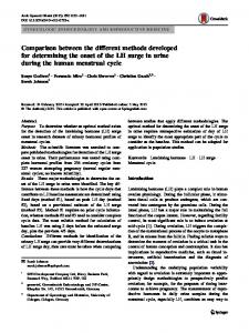
described above are repeated until a stop criterion is reached. In our application, the stop criterion is the mean square error reaching a very low level or the number of epochs reaching a preset value, which ever comes first. An important aspect in modeling the architecture and training of a neural network using DE is coding the neural network. A floating point vector was created that contains all the information from the neural network, as can be seen in Fig.1. In this figure, NL represents the number of hidden layers, the only acceptable values being {0, 1, and 2}. H1 represents the number of neurons in the first hidden layer, H2 the number of neurons in the second hidden layer. The parameters w1, …, wn indicate the weights for each neuron in the neural network, b1, ...., bn the biases and a1, …, an the activation functions. Fig. 1. The content of a solution vector in DE method

In the current application, the fitness function is a combination of MSEtraining and MSEtesting, and the neural network parameters were optimized so that the maximization of the fitness functions is obtained. II. RESULTS AND DISCUSSION By applying the OMP method, a series of simulations were performed using the trial and error method, through the "Vary A Parameter" training process [10], following the algorithm described in section II.B and starting with a single hidden layer neural network. This provided the best network with optimized parameters. Every network was tested using the test data set. Finally, the network with the best performance at training and testing was chosen for further optimization. The heuristic rule (1), applied for a single hidden layer neural network, limited the number of hidden neurons at 105 (H1 ≤ 105). Consequently, the number of neurons in the hidden layer was varied in the interval 5 – 105, with step 5. The maximum number of training epochs was set to 1000. Some of the performance indices obtained through the simulations for optimizing the number of hidden neurons of a single layer neural network are presented in Table I. The best performance was reached for a number of 45 hidden neurons (the last line in Table I). The best number of training epochs found after the cross-validation process was 1000. The learning rates and the momentum terms were varied in the interval 0.1 – 1. The neural network performance obtained after the simulations (average perf_index = 0.8525) did not increase, so the learning rates and the momentum terms were kept to the initial values (1 – the learning rate for hidden layer, 0.1 – the learning rate for the output layer, 0.7 – the momentum term for hidden and output layers). The values of the input data were scaled for the activation function of the hidden layer (the hyperbolic tangent) with values from -0.9 to 0.9. The output values were scaled according to the activation function used for the output layer.

1296

In order for the data used to train and test the neural network to be at the same scale, the values obtained with the simulator for molecular weights were divided by 1000. This is necessary because it was observed that the neural networks cannot learn well if data used for training are not in the same range/scale. TABLE I RESULTS FOR OPTIMIZING THE NUMBER OF HIDDEN NEURONS OF A SINGLE HIDDEN LAYER NEURAL NETWORK Topology / Epochs 20 / 1000 40/ 1000 80/ 1000 45/ 1000

x perf_index 0.9451 0.9388 0.9420 0.94

Mn perf_index 0.8760 0.8787 0.8788 0.8893

Mw perf_index 0.7058 0.7080 0.7107 0.7308

Average perf_index 0.8423 0.8418 0.8439 0.8534

Because the studied problem was a regression problem, and the desired response was a continuous function of the input, the recommended output activation function was the linear function. Nevertheless, the simulations with linear functions did not provide a better performance for the neural network, the maximum average perf_index obtained being 0.8513, whereas the average perf_index of the network before the optimization of the activation function for the output layer was 0.8534. The optimization algorithm ended with the development of an optimized two hidden layers neural network and its comparison with the previous optimized one hidden layer neural networks. For the optimization of the number of hidden neurons in the two hidden layers, the heuristic rules (1) and (3) indicated that H2 ≤ 12. Starting with this statement, taking into acount the number of weights, and applying the "Vary A Parameter" training process, the best two hidden layers neural network proved to be a MLP with 21 neurons in the first hidden layer and 6 neurons in the second hidden layer, with an average perf_index of 0.8772 and 207 weights (the last line in Table II). Some results of the simulations can be observed in Table II. TABLE II RESULTS FOR OPTIMIZING THE NUMBER OF HIDDEN NEURONS OF A TWO HIDDEN LAYERS NEURAL NETWORK Topology / Weights 46 : 9 / 579 15 : 4 / 117 18 : 6 / 180 21 : 6 / 207

x perf_index 0.9642 0.9513 0.9499 0.9579

Mn perf_index 0.9106 0.8884 0.8581 0.8868

Mw perf_index 0.8139 0.7484 0.7584 0.787

Average perf_index 0.8962 0.8627 0.8555 0.8772

Further optimizations on the parameters of the two hidden layers neural network revealed that a learning rate of 0.9 for the first hidden layer, one of 0.2 for the second hidden layer, and a learning rate of 0.07 for the output layer provided an average perf_index of 0.8934. Furthermore, it was observed that a momentum of 0.3 for the first hidden layer and one of 0.7 for the second hidden layer and the output layer, increased the neural network performance to an average perf_index of 0.9060. The simulations for optimizing the activation function for the output layer did not lead to a better performance of the network. The greater average perf_index was obtained for

the linear function, namely 0.8648. By comparing the performance indices obtained for the single hidden layer neural network (average perf_index = 0.8534) and the two hidden layers neural network (average perf_index = 0.9060), respectively, the latter turned out to be the best. The second method applied for developing the topology of a neural network used to model the styrene polymerization process was based on a GA methodology. The results of GA are often influenced by the following parameters: the dimension of initial population (dim_pop), the number of generations (no_gen), the mutation rate (mut_rate), and the crossover rate (cross_rate). The method described in Section C is applied using different values for the GA parameters. Table III shows some neural network topologies obtained by changing these parameters, along with MSE in the training and testing phases. The column “topology” shows the number of neurons in one or two hidden layers. TABLE III NEURAL NETWORK TOPOLOGIES OBTAINED WITH GA METHOD dim no cross mut MSE MSE Topology pop gen rate rate training testing 50 50 0.8 0.2 0.0663 0.1495 16 50 100 0.8 0.2 0.0518 0.1180 15:3 100 50 0.8 0.2 0.0672 0.1267 15:5 100 100 0.8 0.2 0.4629 0.1137 20:7 100 100 0.5 0.2 0.0520 0.1342 15:4 100 100 0.5 0.5 0.0648 0.1302 20:3

The best result was considered a neural network 3:20:7:3 having the smallest error in the testing phase (0.113737; the line marked in bold in Table III). The optimum values found for GA parameters (for which the best neural network was achieved) were dim_pop = 100, no_gen = 100, mut_rate = 0.2, and cross_rate = 0.8. A limitation of the number of hidden neurons was made within our GA: 30 neurons for the first hidden layer and 10 neurons for the second hidden layer were considered enough for the complexity of our problem. The bigger these values, the greater the search space of the GA, but also the greater the search time. The majority of applications from the field of polymerization reactions proved that the maximum number of hidden layers and neurons established in our procedure is enough for obtaining an accurate prediction. In the case of the DE method, the following parameters are used: the crossover factor (cross_rate), the scaling factor (F), and the number of epochs. The efficiency of the algorithm is very sensitive to these parameters [37]. Ilonen et al. [32] consider that F and cross_rate affect the convergence speed and the robustness of the search space, and the optimal values of these parameters depend on the objective function characteristics and the population size parameter. Thus, the determination of the optimal parameter values is dependent on the problem being solved. The role of the cross_rate parameters is to exploit the decomposability property of the problem, in case it exists, and to provide the diversity of the possible solutions. Price et al. [38] showed that all functions could be solved with cross_rate in the range 0 – 2 or 0.9 – 1. We tested cross_rate

1297

by variation of its values in the interval 0.9 – 1. Like cross_rate, the F parameter takes values between 0 and 1, Price et al. [38] considering that F can take values bigger than 1, but it has been observed that no function tested required F > 1. Zaharie [39] demonstrated that a lower limit for F (called Fcritical) exists, in which case the population can converge even if the selection pressure does not exist. In practice F must be greater than Fcritical and, in our case, we tested F between 0.6 and 0.9. The number of epochs represents the generations the algorithm will run. For the values of the epochs that are too low, the results are in local minima. If the values are too high, the computation time of the algorithm is too long but, for 5000 epochs our application had the results in approximately 2.5 hours. As shown in the Table IV, the maximum fitness value was obtained when cross_rate = 0.99, F = 0.7, and the number of epochs = 5000.

representation because of clarity reasons. In these figures, the differences between the desired values and those provided by the neural networks become visible for the individual points of the testing set. Once again, it can be noticed that the three methods give comparable results whose accuracy can be considered very good. TABLE V RELATIVE ERRORS AND CORRELATIONS OBTAINED THROUGH THE THREE METHODS APPLIED FOR DEVELOPING NEURAL NETWORK TOPOLOGIES Average relative Correlations errors (%) x Mn Mw x Mn Mw OMP 0.044 5.480 7.018 0.999 0.989 0.988 3:21:6:3 GA 0.811 2.233 6.130 0.999 0.998 0.994 3:20:7:3 DE 0.787 2.437 6.385 0.999 0.993 0.979 3:9:7:3

TABLE IV RESULTS OF THE SIMULATIONS FOR F=0.7 AND CROSS_RATE=0.99 cross F Epochs Fitness Topology rate 0.99 0.7 500 7.66 10 0.99 0.7 1000 13.55 6 0.99 0.7 2000 16.63 4 0.99 0.7 3000 20.79 4:2 0.99 0.7 4000 25.05 6 0.99 0.7 5000 27.08 9:7

A bigger network can better predict the desired parameters, but a coded bigger network has a bigger vector associated with it, which determines the increase of simulation time. A favorable compromise is reached by limiting the number of nodes in the first hidden layer at 20, and the nodes in the second hidden layer at 10. Different results are obtained with the three methods, thus a comparative evaluation is necessary. Table V presents relative errors obtained by applying the three methods, calculated with the following formula: p − p net E r = desired ⋅100, (8) p desired where pdesired represents x, Mn or Mw as targets of the neural network, and pnet is the prediction of the network for each of the three output variables. Besides errors, Table V also presents the correlations between the data used for testing (a number of 524 data) and the predictions of the three neural networks selected through the three methods (see the first column of the table). Three types of activation functions were used: step, linear and bipolar sigmoid, each being coded using integer numbers. All the networks parameters excluding the number of inputs and outputs are internally changed by the algorithm described above. In the case of integer coded values of the activation function, the algorithm chooses the closest integer values of each of the aa ,…,an parameters contained in the coded vector. Fig. 2, Fig. 3, and Fig. 4 show the testing phase of the three methods based on the same data set. Only 10 data from the testing data set were chosen for the graphical

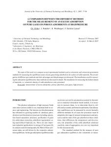
Fig. 2. Some values for conversion: desired vs. obtained conversion in the testing phase through the neural networks designed with the three methods (OMP, GA, DE).

A comparison between these methods will take into account both the error values, but also other factors such as the accessibility of the method (execution time, algorithm complexity etc.) or the purpose to which the model is intended (prediction, monitoring, or control). Fig. 5 shows the variation of monomer conversion and molecular masses with time, obtained with MLP(3:21:6:3) for training and validation data, and demonstrates that neural network modeling is an adequate procedure for rendering the process under study (the critical point where a sudden increase takes place is well modeled). All the three methods have acceptable results in the testing phase, with percent relative errors less than 7%. The three methods have both advantages and disadvantages. DE and GA provide better predictions for the molecular weights, Mn and Mw, whereas the OMP method leads to very small errors for conversion in the testing phase. In terms of accessibility, DE and GA methods, once implemented, are easy to use because the execution of the software program provides the optimal network topology, training and testing errors, and predictions over the training and testing data. However, the runs of the program should be repeated because of the stochastic nature of the algorithms. Furthermore, one cannot say precisely that the results of

1298

these algorithms are optimal networks because there is always the possibility of reaching a local optimum. The parameters of these algorithms control the accuracy of the results, so optimal values have to be chosen for these parameters in order to obtain global optima.

OMP and GA worked better.

Fig. 5. Variation of conversion and molecular masses with time obtained with MLP(3:21:6:3) for training and validation data (validation points are drawn differently for each curve). Fig. 3. Some values for numerical average molecular weight: desired vs. obtained molecular weight in the testing phase through the neural networks designed with the three methods (OMP, GA, DE).

Fig. 4. Some values for gravimetrical average molecular weight: desired vs. obtained molecular weight in the testing phase through the neural networks designed with the three methods (OMP, GA, DE).

The main advantages of DE and GA are the capability to work with noisy or nonlinear functions and the ability to find the global optimum, although the objective function can have multiple local optima. The biggest disadvantage is the fact that they can get stuck in local optima if the correct parameter values are not chosen. The OMP method is more laborious, but the systemized practical considerations on modeling a neural network (structured in a 6-steps algorithm) and the criteria and formula used for calculating the performance indices give this method a real chance to obtain a neural network of minimum size and maximum performance. In addition, the reason of testing three methods was related to the intention of developing a general methodology useful for different applications. Our previous experience showed that the method for obtaining the best neural network topology depends to the set of initial data (type of process). For example, DE method provided better results for classification problems; here, for styrene polymerization,

OMP method was developed in the neural network simulation environment NeuroSolutions, and it is very useful for beginners in neural modeling. It does not require any other knowledge about artificial intelligence tools and it provides the user with total control over the steps of the parameters optimization technique. Moreover, the performance indices formulated for the quantification of the obtained neural network performance outline an effective guideline at every step of the optimization methodology. The two evolutionary methods used for developing the near optimal topology of neural networks (GA and DE) were implemented in C# programming language, and then the programs were integrated into a software product with a graphical user interface. This interface is simple to use, but the user must know the means to find the specific optimal parameters for each problem. The software which implemented the modeling methodologies can be easily extended for different maximum number of intermediate layers and neurons and for other experimental data and applications. III. CONCLUSION The results of this paper will be improved and continued on the following directions: to quantify and classify all NN parameters which define and significantly influence the topology, to test other different objective functions, to improve the effectiveness of the algorithms in finding a NN optimal architecture, and to approach other complex case studies as tests for the developed methods. REFERENCES [1] [2] [3]

1299

F. A. N. Fernandes and L. M. F. Lona, “Neural Network applications in polymerization processes,” Braz. J. Chem. Eng., vol. 22, no. 3, pp. 323-330, 2005. S. Curteanu and C. Petrila „Neural network based modeling for semibatch and nonisothermal free radical polymerization,” Int. J. Quantum Chem., vol. 106, nr.6, pp. 1445-1456, 2006. J. Lobato, P. Cañizares, M. A. Rodrigo, J. J. Linares, C.-G. Piuleac, S. Curteanu, “The neural network based modelling of a PBI-based polymer electrolyte membrane fuel cell: effect of temperature,” J. Power Source, vol. 192, no. 1, pp. 190-194, 2009.

[4]

[5]

[6]

[7] [8]

[9]

[10] [11] [12]

[13] [14] [15] [16] [17]

[18] [19] [20]

[21]

C.-G. Piuleac, M. Rodrigo, P. Cañizares, S. Curteanu, and C. Sáez „Ten steps modelling of electrolysis processes by using neural networks,” Environ. Modell. Softw., vol. 25, no. 1, pp. 74-81, January 2010. P. G. Benardos and G. C. Vosniakos, “Prediction of surface roughness in CNC face milling using neural networks and Taguchi’s design of experiments,” Rob. Comput. Integr. Manuf., vol. 18, pp. 343-354, 2002. W. Sukthomya and J. Tannock, “The optimization of neural network parameters using Taguchi’s design of experiments approach: an application in manufacturing process modeling,” Neural Comput. Appl., vol. 14, pp. 337–344, 2005. S. Sureerattanan and N. Sureerattanan, “New training method and optimal structure of backpropagation networks,” Lect. Notes Cmput. Sci., vol. 3610, pp. 157-166, 2005. E. I. Vlahogianni, M. G. Karlaftis, and J. C. Golias, “Optimized and meta-optimized neural networks for short-term traffic flow prediction: A genetic approach,” Transport. Res. C-Emer., vol. 13, no. 3, pp. 211234, 2005. P. P. Balestrassi, E. Popova, A. P. Paiva, and J. W. Marangon Lima, “Design of experiments on neural network's training for nonlinear time series forecasting,” Neurocomputing, vol. 72, no. 4-6, pp. 11601178, 2009. R. Furtuna, S. Curteanu, and M. Cazacu, „Optimization methodology applied to feed-forward artificial neural network parameters,” Int. J. Quantum Chem., DOI 10.1002/qua.22423, to be published. M. Attik, L. Bougrain, and F. Alexandre, “Neural network topology optimization,” ICANN, vol. 2, pp. 53-58, 2005. S. E. Fahlman and C. Lebiere, “The cascade-correlation learning architecture” in Advances in neural information processing systems, vol. 2, D.S. Touretzky, San Mateo, CA: Morgan Kaufmann, 1990, pp. 524-532. E. Alpaydn, “GAL: Networks that grow when they learn and shrink when they forgot,” ICSI, Berkley, CA, Tech. Rep. TR-91-032, 1991. T. Y. Kwok and D. Y. Yeung, “Constructive algorithms for structure learning in feedforward neural networks for regression problems,” IEEE Trans. Neural Networks, vol. 8, no. 3, pp. 630-645, 1999. L. Ma and K. Khorasani, “New training strategies for constructive neural networks with application to regression problems,” Neural Networks, vol. 17, pp. 589-609, 2004. M. Shahjahan and K. Murase, “A pruning algorithm for training cooperative neural network ensembles,” IEICE Trans. Inf. Syst., E89D(3), pp. 1257-1269, 2006. D. Elizondo, R. Birkenhead, M. Gongora, E. Taillard, and P. Luyima, “Analysis and test of efficient methods for building recursive deterministic perceptron neural networks,” Neural Networks, vol. 20, pp. 1095-1108, 2007. H. J. Xing and B.G. Hu, “Two-phase construction of multilayer perceptrons using information theory,” IEEE Trans. Neural Networks, vol. 20, no. 4, pp. 715-721, 2009. M. Annunziato, I. Bertini, M. Lucchetti, and S. Pizzuti, “Evolving weights and transfer functions in feed forward neural networks,” in Proc. EUNITE2003, Oulu, Finland, 2003. M. Rocha, P. Cortez, and J. Neves, “Simultaneous evolution of neural network topologies and weights for classification and regression,” in IWANN 2005, LNCS 3512, J. Cabestany, A. Prieto, D. F. Sandoval (Eds.), Springer-Verlag Berlin Heidelberg, 2005, pp. 59-66. W. C. Gerken, L. K. Purvis, and R. J. Butera, “Genetic algorithm for optimization and specification of a neuron model,” Neurocomputing, vol. 69, pp. 1039-1042, 2006.

[22] M. Dam and N. D. Saraf, “Design of neural networks using genetic algorithm for on-line property estimation of crude fractionator products,” Comput. Chem. Eng., vol. 30, pp. 722-729, 2006. [23] P. G. Benardos and G. C. Vosniakos, “Optimizing feedforward artificial network architecture,” Eng. Appl. Artif. Intell., vol. 20, no. 3, pp. 365-382, 2007. [24] S. Curteanu and F. Leon, “Optimization strategy based on genetic algorithms and neural networks applied to a polymerization process,” Int. J. Quantum Chem., vol. 108, no.4, pp. 617-630, 2007. [25] M. M. Islam and K. Murase, “A new algorithm to design compact two-hidden-layer artificial neural networks”, Neural Networks, vol. 14, no. 9, pp. 1265-1278, Nov. 2001. [26] S. Curteanu, „Modeling and simulation of free radical polymerization of styrene under semibatch reactor conditions,” Cent. Eur. J. Chem., vol. 1, pp. 69-90, 2003. [27] Y. S. Kim and B. J. Yum, “Robust design of multilayer feedforward neural networks: An experimental approach,” Eng. Appl. Artif. Intell., vol.17, no. 3, pp. 249-263, 2004. [28] M. S. Packianather, P. R Drake, and H. Rowlands, “Optimizing the parameters of multilayered feedforward neural networks through Taguchi design of experiments,” Qual. Reliab. Eng. Int., vol. 16, pp. 461–473, 2000. [29] Q. Wang, D. J. Stockton, and P. Baguley, “Process cost modelling using neural networks,” Int. J. Prod. Res., vol. 38, no. 16, pp. 3811– 3821, 2000. [30] Maren, C. Harston, and R. Pap, Handbook of Neural Computing Applications. Academic Press Inc., San Diego, California, 1990. [31] P. A. Castillo, J. J. Merelo, A. Prieto, V. Rivas, and G. Romero, “GProp: Global optimization of multilayer perceptrons using GAs,” Neurocomputing, vol. 35, pp. 149-163, 2000. [32] J. Ilonen, J. K. Kamarainen, and J. Lampien, “Differential evolution training algorithm for feed-forward neural networks,” Neural Process. Lett., vol. 17, no. 1, pp. 93-105, 2003. [33] P. Plagianakos, G. D. Magoulas, N. K. Nousis, and M. N. Vrahatis, “Training multilayer networks with discrete activation functions,” in Proc. of the INNS-IEEE international joint conference on neural networks, July 2001. [34] B. Subudhi and D. Jena, “Differential evolution and Levenberg Marquardt trained neural networks scheme for nonlinear system identification,” Neural Process. Lett., vol. 27, no. 3, pp. 285-296, 2008. [35] B. Subudhi and D. Jena, “An Improved Differential evolution and Levenberg Marquardt trained neural networks scheme for nonlinear system identification,” Int. J. Autom. Comput., vol. 6, no. 2, pp. 137144, 2009. [36] S. K. Lahiri and N. Khalfe. 2010. “Modeling of commercial ethylene oxide reactor: A hybrid approach by artificial neural network & differential evolution.” Int. J. Chem. Reactor Eng. vol. 8 (A4). Available: http://www.bepress.com/ijcre/vol8/A4. [37] J. Tvrdik, “Adaptive differential dvolution: Application to nonlinear regression,” in Proc. of International Multiconference on Computer Science and Information Technology IMCSIT 2007, M. Ganzha, M. Paprzycki, T. Pelech-Pilichowski (eds), Wisla, Poland, Oct. 2007, pp. 193-202. [38] K. V. Price, R. M. Storm, and J. A. Lampinem, Differential Evolution A Practical Approach to Global Optimization. Springer, 2005. [39] D. Zaharie, “A comparative analysis of crossover variants in differential evolution,” in Proc. of International Multiconference on Computer Science and Information Technology IMCSIT 2007, M. Ganzha, M. Paprzycki, T. Pelech-Pilichowski (eds), Wisla, Poland, Oct. 2007, pp. 171-181.

1300