Comparison between Prediction Capabilities of Neural Network and

Vol. 3 (3) July 2010

Disaster Advances

Comparison between Prediction Capabilities of Neural Network and Fuzzy Logic Techniques for L and Slide Susceptibility Mapping Pradhan Biswajeet 1,2* and Pirasteh Saied 2

1. Institute for Cartography, Faculty of Forestry, Geo and Hydro-Science, Dresden University of Technology, 01062 Dresden, GERMANY 2. Institute for Advanced Technologies (ITMA) University Putra Malaysia, 43400, UPM, Serdang Selangor Darul Ehsan, MALAYSIA *biswajeet24@ gmail.com

presents a comparative study of the application of a neural network and fuzzy logic techniques for L and slide susceptibility mapping in the studied area. A GIS was used as the basic analysis tool for spatial management and data manipulation because of its ability for handling huge amount of spatial data for L and slide analyses.

Abstract Preparation of L and slide susceptibility maps is important for engineering geologists and geomorphologists. However, due to complex nature of L and slides, producing a reliable susceptibility map is not easy. In recent years, various data mining and soft computing techniques are getting popular for the prediction and classification of L and slide susceptibility and hazard mapping. This paper presents a comparative analysis of the prediction capabilities between the neural network and fuzzy logic model for L and slide susceptibility mapping in a geographic information system (GIS) environment. In the first stage, L and slide-related factors such as altitude, slope angle, slope aspect, distance to drainage, distance to road, lithology and normalized difference vegetation index (ndvi) were extracted from topographic and geology and soil maps. Secondly, L and slide locations were identified from the interpretation of aerial photographs, high resolution satellite imageries and extensive field surveys. Then L and slide-susceptibility maps were produced by the application of neural network and fuzzy logic approahc using the aforementioned L and slide related factors. Finally, the results of the analyses were verified using the L and slide location data and compared with the neural network and fuzzy logic models. The validation results showed that the neural network model (accuracy is 88%) is better in prediction than fuzzy logic (accuracy is 84%) models. Results show that “gamma” operator (λ = 0.9) showed the best accuracy (84%) while “or” operator showed the worst accuracy (66%).

In the literature, there have been many studies carried out on L and slide susceptibility and hazard evaluation using GIS. Recently, there have been studies on L and slide hazard evaluation using GIS and many of these studies have applied probabilistic models 4-,7,1113,15,16,19,20,22,25-,27,36-39,40,42,43, 47 . One of the statistical models available, the logistic regression model, has also been applied to L and slide hazard mapping 10,14,18,21,28,31,32,41. There are other methods for L and slide hazard mapping, such as the geotechnical model and the factor of safety model also seen in the literature8. Recently, various data mining and soft computing techniques such as fuzzy logic and artificial neural network approaches have been seen in the L and slide susceptibility mapping literature 1,3,8,17, 22,23,25,29,30,31,32,34 .

Application Site Characteristics The study area has a historical record of L and slides and was selected as a suitable application site for the application of neuro-fuzzy model on L and slide susceptibility mapping. Tanah Rata is located in the central part of Cameron High L ands (Figure 1). The application site covers an area of 24.7 km2. The bedrock geology of the study area consists mainly of megacrystic biotite granite31. L and slides may be classified by type and material. In this area, most of the L and slides were shallow soil slides and debris flows that occurred where the maximum daily rainfall was between 87-100 mm31-33. A key assumption of our approach was that potential events (occurrence probability) would be represented by this distribution of L and slides. An ArcGIS 9.0 (ESRI, Redl ands, CA, USA) was used as the basic analysis tool for spatial management and data manipulation and MatLab 7.1 software (The Math Works, Inc., Natick, MA, USA) was used for neural network and fuzzy logic processing31.

Keywords: Neural network, fuzzy logic, data mining, L and slide, susceptibility, GIS, remote sensing, Malaysia.

Introduction Frequent L and slides pose a significant risk in Malaysia, causing damage that affects people and property almost every year29. Much damage was caused on such occasions in the study area of Tanah Rata. Through scientific analysis, it is possible to identify and evaluate susceptible areas in order to reduce the hazard by proper engineering adaptation to the slope stability. This paper

Spatial Datasets Used For the L and slide-susceptibility mapping, the main steps were data collection and construction of a spatial database from which the relevant factors were extracted, followed by assessment of the L and slide (26)

Vol. 3 (3) July 2010

Disaster Advances susceptibility using the relationship between L and slide and L and slide-related factors and validation of the results. A key assumption of this approach was that the potential (occurrence probability) of L and slides would be comparable to the actual frequency of L and slides. L and slide occurrence areas were detected in the Cameron hill area by interpretation of aerial photographs, high resolution satellite images, inventories and field surveys. A map of recent L and slides was developed from 1:20 000 scale aerial photographs and was used to evaluate the frequency and distribution of shallow L and slides in the area. Topography, geology and lineament databases were constructed for the analysis (Table 1). Maps relevant to L and slide occurrence were constructed from a vector-type spatial database using Arc/Info GIS software (ESRI). These included 1:25,000 scale topographic maps (National Mapping Agency, Malaysia) and 1:63,600 scale geology maps (Department of Geology and Mineral Mapping, Malaysia).

aspect and plan curvature was extracted from the DEM, distance to drainage was calculated from the drainage database; distance to road was calculated from topography map; and lithology and distance from fault was extracted from the geological database. A L and cover map was prepared from the SPOT 5 satellite image using a supervised classification. Further, normalized difference vegetation index map (ndvi) was extracted from the L ANDSAT TM image. Using the detected L and slide locations and the constructed spatial database, L and slide analysis methods were applied and validated. For this aim, the calculated and extracted factors were mapped to a 10 m x 10 m grid in Arc/Info GRID format. Next, using the likelihood ratio, fuzzy logic and ANN approach, spatial relationships between the L and slide location and each of the L and slide-related factors, such as altitude, slope angle, slope aspect, plan curvature, distance to drainage, distance to road, lithology, L and cover and normalized difference vegetation index (ndvi) were analyzed.

A digital elevation model (DEM) was created using the topographic database. Altitude, slope angle, slope

Figure 1: Study area showing hill shaded DEM L and slide location map.

(27)

Vol. 3 (3) July 2010

Disaster Advances

Error

Ep =

C

o11 y11

1 2

m

∑(y

p j

− o jp ) 2

j =1

o21 y21

Output layer

To t nodes in layer q+1

O = O (V )

l

Hidden layer

v

Node j in layer q

q, p j =

∑ω k =1

h, j

o

p h

ω n, j From l nodes in layer q-1 Input layer

A x11

x21

x31

SPATIAL DATABASE

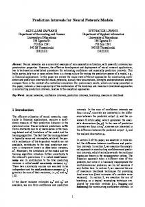
Figure 2: Three tiered architecture of feed-forward, back-propagation neural network (multilayer perception). (A): The presentation of training input data layer pattern 1with the values of x1, x2, and x3 . (B) The output values of the network (o1 and o2) . (C): The desired output pattern for the first samples of the training data (y1 and y2) 24.

Data layers Land slide inventory

Topographic map Geological map Drainage Land cover Vegetation Index (NDVI)

Table 1 Thematic layers used in this study Data type Source of data Polygon coverage Land slide inventory database, aerial photos, field surveys Line and Point coverage National Mapping Agency Polygon coverage Minerals and Geoscience Department Line coverage Department of Agriculture GRID Landsat TM images GRID SPOT 5 image

to describe particular models24. First, unlike expert systems, ANNs are not initialized with any external rule base. Rather the goal of the ANN is to internally identify a set of rules for matching input data to output conclusions. An ANN is composed of a set of nodes and a number of interconnected processing elements. ANN uses learning algorithms to model knowledge and save this knowledge in weighted connections, mimicking the function of a human brain24. One of the most commonly used ANN models is the feed-forward back-propagation ANN. This is a supervised, pattern recognition model that needs to be trained using a data set for which both the input values (x) for a set of predictors and the correct output values (y) are known for a set of examples.

Theory: Artificial Neural Network (ANN) The artificial neural network approach has many advantages compared with other statistical methods. First, the artificial neural network method is independent of the statistical distribution of the data and there is no need for specific statistical variables. Neural networks allow the target classes to be defined in relation to their distribution in the corresponding domain of each data source24 and therefore integration of remote sensing data or GIS data is convenient. An artificial neural network is a “computational mechanism able to acquire, represent and compute a mapping from one multivariate space of information to another, given a set of data representing that mapping”46. Most ANN models share a number of characteristics. These will be identified before proceeding (28)

Vol. 3 (3) July 2010

Disaster Advances

implemented with a GIS modelling language. This is different from data-driven approaches such as weights of evidence or logistic regression, which use the locations of known objects such as L and slides to estimate weights or coefficients. The idea of using fuzzy logic in L and slide hazard mapping is to consider the spatial objects on a map as members of a set. For example, the spatial objects could be areas on an evidence map and the set defined as ‘areas hazardous to L and slide’. Fuzzy membership values must lie in the range (0, 1), but there are no practical constraints on the choice of the fuzzy membership values. Values are chosen to reflect the degree of membership of a set, based on subjective judgment. Given two or more maps with fuzzy membership functions for the same set, a variety of operators can be employed to combine the membership values.

The architecture of this ANN is based on a structure known as the Multi-Layer Perceptron (MLP). The MLP, as the name implies, consists of a set of layers, each of which is composed of a set of nodes (alternatively referred to as “processing elements”, “units”, “processing units”, or “neurons”). The MLP with the back-propagation algorithm is trained using a set of examples of associated input and output values. This learning MLP algorithm is trained with the “Back-Propagation algorithm”, which consists of an input layer, hidden layer and an output layer (Figure 3). The detail about the ANN can be seen in Moody and Katz24. The first layer of the network, or input layer, contains a node for each of input variables (Figure 3). The input variables are analogous to the independent variables in multiple regressions. When a given set of input values for one of the n samples in the training data set is presented to the input nodes, we say that the network is presented with an input pattern (where to). The superscript indicates terms that consists of or refer to a given pattern of values24.

Zimmerman45 discussed a variety of combination rules. Bonham-Carter2 discussed five operators, namely the fuzzy and, fuzzy or, fuzzy algebraic product, fuzzy algebraic sum and fuzzy gamma operator. This study uses the five fuzzy operators for combining the fuzzy membership functions.

The last layer of the network, or output layer, contains nodes resembling one for each output type (Figure 3). In this case, there are eleven input nodes (one each for altitude, slope angle, slope aspect, plan curvature, distance to drainage, distance to road, lithology, L and cover and ndvi) and the output layer will have one node. Sandwiched between the input and output layers is one “hidden” layer which will allow complexities to develop in the mapping functions. In this case, a three tired ANN architecture model is used. The hidden layer, like the input and output layer, consists of nodes.

Like the membership function, the frequency ratio was calculated. The frequency ratio is shown in table 2 for all factors. The spatial relationships between the L and slide location and each L and slide-related factor were analyzed by using the probability model–frequency ratio. The frequency ratio, a ratio between the occurrence and absence of L and slides in each cell, was calculated for each factor’s type or range that had been identified as significant with respect to causing L and slides. An area ratio for each factor’s type or range to the total area was calculated. Finally, frequency ratios for each factor’s type or range were calculated by dividing the L and slide occurrence ratio by the area ratio. If the ratio is greater than 1, the relationship between L and slides and the factors is higher and, if the ratio is less than 1, the relationship between L and slide and each factor’s type or range is lower. Then, the frequency ratio was normalized between 0.00 and 1.00 to create the fuzzy membership value.

Theory: Fuzzy logic operators

The fuzzy set theory introduced by Zadeh44 is one of the tools used to handle the complex problems. Therefore, the fuzzy set theory has been commonly used for many scientific studies in different disciplines. The idea of fuzzy logic is to consider the spatial objects on a map as members of a set. In the classical set theory, an object is a member of a set if it has a membership value of 1, or is not a member if it has a membership value of 0. In the fuzzy set theory, membership can take on any value between 0 and 1 reflecting the degree of certainty of membership. The fuzzy set theory employs the idea of a membership function that expresses the degree of membership with respect to some attribute of interest.

ANN to L and slide susceptibility mapping: The L and slide-related factors such as altitude, slope angle, slope aspect, distance to drainage and distance to road, lithology and ndvi were converted from vector-type data to grid-type data with 10 m grids. The continuous-type grid data, such as altitude, slope angle, distance to drainage, distance to road and ndvi were reclassified to make categorical-type grid data using the equal area classification method, in which each zone represents a similar amount of area. All the grid type data had 497 rows and 497 columns.

With maps, generally, the attribute of interest is measured over discrete intervals and the membership function can be expressed as a table relating map classes to membership values. Fuzzy logic is attractive because it is straightforward to understand and implement. It can be used with data from any measurement scale and the weighting of evidence is controlled entirely by the expert. The fuzzy logic method allows for more flexible combinations of weighted maps and could be readily

For analysis of L and slide susceptibility, the training sites were selected from the L and slide-related factors and the back propagation algorithm was applied to calculate weights between the input layer and the hidden (29)

Vol. 3 (3) July 2010

Disaster Advances

0.4, 0.5, 0.6, 0.7, 0.8, 0.9, 0.95 and 0.975 in order to detect its effect on the L and slide susceptibility map.

layer and between the hidden layer and the output layer, by modifying the number of hidden layers and the learning rate. The weights were applied to the entire study area and the L and slide susceptibility index values were calculated. The calculated index values were converted into an ARC/INFO GRID using the GIS. Then the L and slide susceptibility map was created using the GRID data. A three-layered feed forward network was implemented in MATLAB. Feed-forward means that all the interconnections between the layers propagate forward to the next layer. The number of hidden layers and the number of nodes in a hidden layer required for a particular classification problem are not easy to deduce. In the study, the structure 9 (input layer) × 19 (hidden layer) × 1 (output layer) were selected for the network with input data normalized to the range 0.1 to 0.9. The nominal and interval class group data were converted to continuous value between 0.1 and 0.9. The content of the number is not considered in the process of the calculation using the neural network program, but the number used to distinguish the classes of each factor in the process of the calculation using artificial neural network program. Therefore, the continuous value is not ordinal data but nominal data and the numbers refer to the classification of the input data.

Figure 3: Distribution of training samples during the ANN modelling

Using the fuzzy membership function (Fig. 5) and the fuzzy operator, the L and slide susceptibility index (LSI) values were computed for the 17 cases including the 13 cases in which the gamma operator was used. The computed LSI values were mapped to allow interpretation such as that illustrated for example in the case of fuzzy membership “gamma operator” (Fig. 6). The values were classified into equal areas and grouped into five classes for visual interpretation. For example, in the case of applying the fuzzy and product, the minimum, mean, maximum and standard deviation values of each LHI are 0.00, 0115, 0.3311 and 0.0278 respectively. In the case of applying the fuzzy algebraic sum, the minimum, mean, maximum and standard deviation values of each LSI are 0.0039, 0.0289, 0.0543 and 0.0086 respectively. In the case of applying the gamma operator (λ = 0.975), the minimum, mean, maximum and standard deviation values of each LSI are 0.000, 0.3008, 1.6985 and 0.6137 respectively. Also, in the case of applying the gamma operator (λ = 0.8), the minimum, mean, maximum and standard deviation values of each LSI are 0.000, 0.079, 0.00084 and 0.00114 respectively.

The learning rate was set to be 0.01 and the initial weights were randomly selected. The initial weights were set between 0.1 and 0.3 automatically. To test whether the variation of weights is dependent on initial weight or not, the weights which were calculated from many cases were compared. The results revealed that the initial weight did not influence the weight in the condition. From each of the two classes (L and slide and not-L and slide), all L and slide occurrence and flat pixels for each study area were used for training data. The distribution of the training samples is shown in fig. 3. The selected L and slide prone locations were assigned (0.1, 0.9) and the no prone L and slide locations were assigned (0.9, 0.1). To lessen the error between the predicted output values and actually calculated output values, the back propagation algorithm was used. The algorithm propagates the weights backwards and then controls the weights. The numbers of epochs were set to 2,00 and Root Mean Square Error (RMSE) goal for stopping criterion was set to 0.01. All of the iteration met the 0.01 root mean square error goal less than 300 epochs. The susceptibility map produced by the neural network technique is shown in fig. 4.

Verification of the susceptibility maps by ROC method: For verification of L and slide hazard calculation methods, two basic assumptions are needed. One is that L and slides are related to spatial information such as topography, geology, the location of lineaments and the other is that future L and slides will be precipitated by a specific impact factor, such as rainfall or an earthquake4. The success rate illustrates how well the estimators perform. To obtain the relative ranks of each L and slide hazard index, the calculated index values of all cells in the study area were sorted in descending order. Then, the ordered cell values were divided into 100 classes with accumulated 1% intervals (Fig. 7).

Fuzzy logic operators to L and slide susceptibility mapping: The input L and slide related factors were combined for assigning membership functions. These seven factors were combined to generate the L and slide susceptibility map using fuzzy operators such as fuzzy and, fuzzy or, fuzzy algebraic product, fuzzy algebraic sum and fuzzy gamma operator. In the case of fuzzy gamma operator, the value of λ was set to 0.025, 0.05, 0.1, 0.2, 0.3, (30)

Vol. 3 (3) July 2010

Disaster Advances

Figure 4: Land slide susceptibility map based on ANN model.

processed in the GIS environment quickly and easily. The ANN model requires conversion of the data to ASCII or other formats for use in the MATLAB package and later reconversion to incorporate it into the GIS database. Similarly, in the case of a both ANN and fuzzy logic model, the factors must have a normal distribution. In other words, the dependent variable must be input as 0 or 1, for L and slide susceptibility analysis. The L and slide susceptibility maps produced by ANN and fuzzy logic approaches can be used for generalization and planning purpose. The maps are easy to understand and interpret.

For verification of predictive maps using the neural network and fuzzy logic approaches, the success rate and area under curves (AUC) of the success rate curves were computed (Fig. 7). The verification results show that L and slide susceptibility map produced by neural network approach had better prediction capacity (88%) than the one produced by the fuzzy logic operator (84%).

Conclusion This paper demonstrates a comparative analysis of ANN and fuzzy logic technique for L and slide susceptibility mapping in a GIS environment. First, L and slide locations were identified from the interpretation of aerial photographs and field survey and L and slide-related factors such as altitude, slope angle, slope aspect, plan curvature, distance to drainage, distance to road, lithology, L and cover and ndvi were used as input data for the modeling of ANN and fuzzy logic techniques. The resultant L and slide susceptibility maps were further verified using the L and slide test data which were not used during the training of the models. The verification results showed that, ANN technique has better accuracy than the fuzzy logic approach for the studied area.

References 1. Atkinson P.M. and Massari R., Generalized linear modeling of susceptibility to L and sliding in the central Apennines, Italy, Computer & Geosciences 24, 373-385 (1998) 2. Bonham-Carter G.F., Geographic Information Systems for Geoscientists, Modelling with GIS (1994) 3. Choi J., Oh H.J., Lee S., Won J.S. and Lee S., Validation of an artificial neural network model for L and slide susceptibility mapping, Environmental Geology, Online published (2009) 4. Chung C.F. and Fabbri A.G., Probabilistic prediction models for L and slide hazard mapping, Photogrammetric Engineering & Remote Sensing, 65, 1389-1399 (1999)

The ANN modeling technique has the advantage of the expert knowledge and learning capability of fuzzy logic, but gradient descent still slows down the training process and the training time could be prohibitively long for a complicated task. In this study, both the data mining approaches (ANN and fuzzy logic) were used. As a result, the soft computing technique is shown to be useful for L and slide susceptibility mapping. The fuzzy logic model is simple and the process of input, calculation and output can be readily understood. The large amount of data can be

5. Clerici A. et al, A GIS-based automated procedure for L and slide susceptibility mapping by the Conditional Analysis method: the Baganza valley case study (Italian Northern Apennines), Environmental Geology, 50, 941-961 (2006) 6. Dahal R.K. et al, GIS-based weights-of-evidence modelling of rainfall-induced L and slides in small catchments for L and slide susceptibility mapping, Environmental Geology, 54, 311 (2008)

(31)

Vol. 3 (3) July 2010

1,60

14

1,40

12

1,20

10

1,00

8

0,80

6

0,60

4

0,40

2

0,20

0

0,00

50

8,00 7,00

40

6,00 5,00

30

FR

1,80

16

F r e q u e n c y (% )

18

FR

F r e q u e n c y (% )

Disaster Advances

4,00 20

3,00 2,00

10

1,00 0

0,00

[1260 ~ [1457 ~ [1491 ~ [1529 ~ [1561 ~ [1590 ~ [1616 ~ [1642 ~ [1680 ~ [> 1733] 1456) 1490) 1528) 1560) 1589) 1615) 1641) 1679) 1732)

0 - 15°

16 - 25°

26 - 35°

> 36°

(b) Slope angle in degrees

(a) Altitude (m) 25

90

2,00

2,50

80

15 1,00 10 0,50

5 0 N

NE

E

SE

S

SW

W

60 1,50

50 40

1,00

30 20

0,50

10

0,00 Flat

2,00

70

FR

F r e q u e n c y (% )

1,50

FR

F r e q u e n c y (% )

20

0

NW

0,00 Concave

(c) Slope aspect

Flat

Convex

(d) Plan curvature 2,40

25

1,20

1,20 10

0,80

5

0,40

0

0,00 [0-91) [92 ~183) [184 ~ 275)

[276 ~ 367)

[368 ~ 458)

[459 ~ 550)

[551 ~ 642)

[643 ~ 734)

[735 ~ 826)

80 0,80

60

FR

F req u en cy (% )

1,60

15

FR

40

0,40

20 0

[> 826]

0,00 Acid intrusives (undifferentiated)

(f) Lithology 2,00

80

4,00

16

1,60

60

3,00

12

1,20

40

2,00

8

0,80

4

0,40

20

1,00

0

0

0,00 [0 ~ 78)

[80 ~ 160)

[161 ~ 246)

[247 ~ 342)

[343 ~ 451)

[452 ~ 590)

[591 ~ 776)

[777 ~ 1045)

Frequency (% )

20

FR

F req u en cy ratio (% )

(e) Distance to drainage (m)

Schist, phyllite, slate and limestone. Minor intercalations of sandstone and volcanics

0,00 PRI_FOREST

[1046 ~ [> 1551] 1551)

CUTTING

GRASS

RUBBER

WATER BODY

(h) Landcover

(g) Distance to faults (m)

F req u en cy (% )

SEC_FOREST SETTLEMENT

18

1,80

16

1,60

14

1,40

12

1,20

10

1,00

8

0,80

6

0,60

4

0,40

2

0,20

0

Study area landslide area Frequency ratio value (FR) FR

F req u en cy (% )

100

2,00

20

0,00 [-0.783 ~ [-0.605 ~ [-0.428 ~ [-0.251 ~ [-0.073 ~ [0.104 ~ [0.282 ~ [0.459 ~ [0.636 ~ [> 0.814] 0.605) -0.428) -0.251) -0.073) 0.104) 0.282) 0.459) 0.636) 0.814)

(i) ndvi

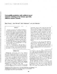
Figure 5: Distribution of landslide related factors for the study area from a representative sample of 247,009 grid cells throughout the study area. Factors are classified using a priori information and their frequency ratio values to landslide occurrences (FR), also shown in the histograms, obtained by likelihood frequency ratio model. (32)

Vol. 3 (3) July 2010

Disaster Advances

Figure 6: Land slide susceptibility map based on fuzzy gamma operator model; using λ = 0.975 Cumulative percentage of of landslide occurrence Cumulative percentage landslide occurrence

100

relationship between tectonic fractures and L and slides, Environmental Geology, 48, 778-787 (2005)

90 80

12. Lee S. and Lee M.J., Detecting L and slide location using KOMPSAT 1 and its application to L and slide-susceptibility mapping at the Gangneung area, Korea, Advances in Space Research, 38, 2261-2271 (2006)

70 60 50

13. Lee S. and Pradhan B., Probabilistic L and slide risk mapping at Penang Isl and, Malaysia, Journal of Earth System Science, 115(6), 661-672 (2006)

40 30

ANN (AUC=89)

20

Fuzzy gamma 0.975 (AUC=84)

14. Lee S. and Pradhan B., L and slide hazard mapping at Selangor, Malaysia using frequency ratio and logistic regression models, L and slides, 4, 33-41 (2007)

10 0 0

10

20

30

40

50

60

70

80

90

100

Landslide susceptibility susceptibility index rank (%) (%) Landslide rank

Figure 7: ROC plot for the land slide susceptibility maps produced by ANFIS showing the cumulative land slide occurrence (%; y-axis) occurring in the land slide susceptibility index rank (%; x-axis).

15. Lee S. and Sambath T., L and slide susceptibility mapping in the Damrei Romel area, Cambodia using frequency ratio and logistic regression models, Environmental Geology, 50, 847-855 (2006) 16. Lee S. and Talib J.A., Probabilistic L and slide susceptibility and factor effect analysis, Environmental Geology, 47, 982-990 (2005)

7. Dai F.C. and Lee C.F., L and slide characteristics and slope instability modeling using GIS, Lantau Island Hong Kong, Geomorphology, 42, 213-228 (2002)

17. Lee S., Application and verification of fuzzy algebraic operators to L and slide susceptibility mapping, Environmental Geology, 52, 615-623 (2007)

8. Ercanoglu M. and Gokceoglu C., Assessment of L and slide susceptibility for a L and slide-prone area (north of Yenice, NW Turkye) by fuzzy approach, Environmental Geology, 41, 720-730 (2002)

18. Lee S., Application of logistic regression model and its validation for L and slide susceptibility mapping using GIS and remote sensing data, International Journal of Remote Sensing, 26, 1477-1491 (2005)

9. Gokceoglu C., Sonmez H. and Ercanoglu M., Discontinuity controlled probabilistic slope failure risk maps of the Altindag (settlement) region in Turkey, Engineering Geology, 55, 277-296 (2000)

19. Lee S., Choi J. and Min K., L and slide susceptibility analysis and verification using the Bayesian probability model, Environmental Geology, 43, 120-131 (2002)

10. Lamelas M.T., Marinoni O., Hoppe A. and Riva J., Doline probability map using logistic regression and GIS technology in the central Ebro Basin (Spain), Environmental Geology, 54, 963977 (2008)

20. Lee S., Choi J. and Min K., Probabilistic L and slide Hazard Mapping using GIS and Remote Sensing Data at Boeun, Korea, International Journal of Remote Sensing, 25, 2037-2052 (2004)

11. Lee S. and Dan N.T., Probabilistic L and slide susceptibility mapping in the Lai Chau province of Vietnam: focus on the

(33)

Vol. 3 (3) July 2010

Disaster Advances 21. Lee S., Comparison of L and slide susceptibility maps generated through multiple logistic regression for three test areas in Korea, Earth Surface Processes and L and forms, 32, 21332148 (2007)

34. Pradhan B., Lee S. and Buchroithner M.F., A GIS-based back-propagation neural network model and its cross application and validation for L and slide susceptibility analyses, Computers Environment and Urban Systems, 34, 216-235 (2010)

22. Lee S., Ryu J.H. and Kim I.S., L and slide susceptibility analysis and its verification using likelihood ratio, logistic regression and artificial neural network models: case study of Youngin, Korea, L and slide, 4, 327-338 (2007)

35. Pradhan B., Lee S. and Buchroithner M., Remote sensing and GIS-based L and slide susceptibility analysis and its crossvalidation in three test areas using a frequency ratio model, Photogrammetrie, Fernerkundung, GeoInformation, 1, 17-32 DOI:10.1127/1432-8364/2010/0037 (2010)

23. Lee S., Ryu J.H., Lee M.J. and Won J.S., L and slide susceptibility analysis using artificial neural network at Boeun, Korea, Environmental Geology, 44, 820-833 (2003)

36. Pradhan, B., Singh R.P. and Buchroithner M.F., Estimation of stress and its use in evaluation of L and slide prone regions using remote sensing data, Advances in Space Research, 37,698 (2006)

24. Moody A. and Katz D. B., Artificial intelligence in the study of mountain L and scapes. In Bishop M. P. and Shorder J. F., (Editors), Geographic information science and mountain geomorphology, Springer, 219-249 (2003)

37. Refice A. and Capolongo D., Probabilistic modeling of uncertainties in earthquake-induced L and slide hazard assessment, Computer and Geosciences, 28, 735-749 (2002)

25. Oh H.J. et al, Predictive L and slide susceptibility mapping using spatial information in the Pechabun area of Thailand, Environmental Geology, 57, 641-651 (2009)

38. Romeo R., Seismically induced L and slide displacements: a predictive model, Engineering Geology, 58, 337-351 (2000) 39. Rowbotham, D. and Dudycha, D.N., GIS modeling of slope stability in Phewa Tal watershed, Nepal, Geomorphology, 26, 151-170 (1998)

26. Ozdemir A., L and slide susceptibility mapping of vicinity of

Yaka L and slide (Gelendost, Turkey) using conditional probability approach in GIS, Environmental Geology, 57, 16751686 (2009)

40. Saied P., Biswajeet P. and Amir M., Stability Mapping and L and slide Recognition in Zagros Mountain South West Iran: A Case Study, Disaster Advances, 2 (1), 47-53 (2009)

27. Pandey A. et al, and L and slide hazard zonation using remote sensing and GIS: A case study of Dikrong river basin, Arunachal Pradesh, India, Environmental Geology, 54, 1517 (2008)

41. Tunusluoglu M.C., Gokceoglu C., Nefeslioglu H.A. and Sonmez H., Extraction of potential debris source areas by logistic regression technique: a case study from Barla, Besparmak and Kapi mountains (NW Taurids, Turkey), Environmental Geology, 54, 9-22 (2008)

28. Pradhan B., Remote sensing and GIS-based L and slide hazard analysis and cross-validation using multivariate logistic regression model on three test areas in Malaysia, Advances in Space Research, 45(10), 1244-1256 (2010)

42. Vijith H. and Madhu G., Estimating potential L and slide

29. Pradhan B. and Lee S., Utilization of optical remote sensing data and GIS tools for regional L and slide hazard analysis by using an artificial neural network model at Selangor, Malaysia, Earth Science Frontiers, 14 (6), 143-152 (2008)

sites of an up L and sub-watershed in Western Ghat's of Kerala (India) through frequency ratio and GIS, Environmental Geology, 55, 1397-1405 (2009) 43. Wang H.B. and Sassa K., Comparative evaluation of L and slide susceptibility in Minamata area, Japan, Environmental Geology 47, 956-966 (2005)

30. Pradhan B. and Lee S., L and slide risk analysis using artificial neural network model focusing on different training sites, International Journal of Physical Science, 3 (11),1 (2009)

44. Zadeh L.A., Fuzzy sets. Information and Control 8, 338(1965) 31. Pradhan B. and Lee S., Delineation of L and slide hazard areas on Penang Isl and, Malaysia, by using frequency ratio, logistic regression and artificial neural network models, Environmental Earth Sciences, Doi: 10.1007/s12665-009-0245-8 60, 1054 (2010)

45. Zimmerman H.Z., Fuzzy Sets Theory and Its Applications, Kluwer Academic Publishers, Dordrecht (1996) 46. Zhou W., Verification of the nonparametric characteristics of back propagation neural networks for image classification, IEEE Transaction on Geoscience and Remote Sensing, 38, 771 (1999)

32. Pradhan B. and Lee S., L and slide susceptibility assessment and factor effect analysis: backpropagation artificial neural networks and their comparison with frequency ratio and bivariate logistic regression modelling, Environmental Modelling and Software, 25(6), 747-759 (2010)

47. Zhou G., Esaki T., Mitani Y., Xie M. and Mori J., Spatial probabilistic modeling of slope failure using an integrated GIS Monte Carlo simulation approach, Engineering Geology, 68, 373386 (2003).

33. Pradhan B. and Lee S., Regional L and slide susceptibility analysis using backpropagation neural network model at Cameron Highland, Malaysia, L and slides, 7(1), 13-30 (2010)

(Received 2nd May 2010, accepted 25th June 2010)

Be Fellow Member of Disaster Advances (34)