Comparison between two numerical methods for a magnetostatic ...

Comparison between two numerical methods for a magnetostatic problem J.-F. Gerbeau, C. Le Bris

CERMICS, Ecole Nationale des Ponts et Chaussées. 6-8 av. Blaise Pascal Cité Descartes - Champs-sur-Marne 77455 Marne-La-Vallée (France)

Abstract

We draw a comparison between two numerical methods to solve a magnetostatic problem set on a bounded convex domain. The problem is of vector Poisson type and is associated with boundary conditions set on the curl of the unknown, here the magnetic eld. These boundary conditions therefore introduce a coupling between the components. One of the two algorithms under consideration consists in an adaptation of the inuence matrix method introduced by R. Glowinski and O. Pironneau [4] on the biharmonic equation and extended later by L. Quartapelle et al [7], [8], [9]. We present a detailed description of the practical implementation of the algorithm. Through various numerical tests, we compare this uncoupled method with a strategy consisting of a direct attack of the coupled problem.

Résumé

Nous comparons deux méthodes numériques pour résoudre un problème de magnétostatique posé sur un domaine convexe borné. Il s'agit d'un problème de Poisson vectoriel dont les conditions aux limites sont posées sur le rotationel de l'inconnu, ici le champ magnétique. Ces conditions aux limites couplent donc les composantes du vecteur inconnu. L'un des deux algorithmes considérés est une adaptation de la méthode des matrices d'inuence introduite par R. Glowinski et O. Pironneau [4] pour le problème du bi-laplacien et étendue ensuite par L. Quartapelle et al [7], [8], [9]. Nous présentons une description détaillée de l'implémentation pratique de l'algorithme. Nous comparons à travers divers tests numériques cette méthode découplée avec une résolution directe du problème couplé.

1 Introduction In this article, we consider a magnetostatic problem set on a bounded convex domain of R 3 , enclosed in a C 1;1 boundary . The magnetic eld B we 1

seek is the solution to a vector Poisson problem with non-classical boundary conditions, namely a system of the form 8 curl (curl B) = f > < div B = 0 (1.1) curl B  n = k  n on > : B:n = q on : It can be seen on (1.1) that the boundary conditions on curl B  n, very natural from the physical standpoint, introduce a coupling between the components of B which prevents one from solving the vectorial problem as three scalar Poisson equations, contrarily to the case when there are three Dirichlet boundary conditions. Some diculties are therefore likely to be encountered from a computational viewpoint. Indeed, whereas in the case of a classical vector Poisson problem, three linear systems of size N 2 have to be solved (N denotes the number of degrees of freedom on the mesh), a coupled system is here to be solved, which increases the required memory. Let us point out that such a situation also occurs in the framework of hydrodynamics when a vector potential associated to the velocity eld in incompressible ows is computed. In this latter context, the system is 8 4 u = f; < n on ; (1.2) : udiv nu == ab  on : In order to solve (1.2) L. Quartapelle and coworkers have extended and analysed an interesting uncoupled algorithm (see [7], [8], [9]) based on the inuence matrix method introduced by R. Glowinski and O. Pironneau. The idea is basically to transform system (1.2) into the resolution of a standard system with Dirichlet boundary conditions together with the resolution of a problem on the surface . From the computational viewpoint, this strategy replaces the resolution of the original linear system by linear systems of smaller size N 2 . The boundary conditions on the vector Poisson equations are dierent in magnetostatics from the ones used in hydrodynamics, but we show in the present work that this algorithm may however be extended in order to treat the magnetostatic problem. Our aim is to compare the following two strategies to solve problem (1.1) :  a direct method which treats simultaneously the three components of B ,  an uncoupled method, following the ideas of Glowinski-Pironneau and Quartapelle and coworkers, which treats successively the three components of B . 2

Let us briey derivate the magnetostatic equation we shall consider henceforth. We begin with the stationary Maxwell equations : curl (B=) = j; (1.3) div B = 0; (1.4) curl E = 0: (1.5) While the magnetostatic problem (1.3)-(1.4) is often solved numerically through the introduction of the so-called scalar and vector potentials (see for instance E. Emson [2] and the bibliography therein), we shall not follow this approach here. In the sequel,  is supposed to be constant, thus we may set  = 1 without loss of generality. On the boundary , we specify some components of the magnetic and electric elds as follows : B:nj = q;

E  nj = 1 k: where n is the outward-pointing normal to . Using the Ohm's law j = E (or j = (E + u  B ) with uj = 0 for a magnetohydrodynamics ow), the boundary conditions on E also reads

curl B  n = 1 k  n:   Let us denote j= by g in the sequel. Taking the curl of (1.3) we obtain the system 1

in ; (1.6) curl ( 1 curl B ) = curl g  div B = 0 in ; (1.7) 1 curl B  n = 1 k  n on ; (1.8)   B:n = q on : (1.9) We suppose that the conductivity  is constant over the domain (see however Remark 5.1 below) and we set  = 1. Therefore, the equations to be solved are : curl (curl B ) = f in ; (1.10) div B = 0 in ; (1.11) curl B  n = k  n on ; (1.12) B:n = q on ; (1.13) 3

where f = curl g. We shall proceed as follows. We study in Section 2 two variational formulations of (1.1). The formulation presented in 2.2 will be used in the uncoupled strategy whereas the formulation of Section 2.3 will be used in the direct method. The two approaches are then detailed in Sections 3 and 4. We compare the results obtained with the two methods in Section 5 in term of precision, CPU time and memory. Finally, in Section 6 we draw conclusions about our whole work.

2 Variational formulations We present in this section two variational formulations of (1.10)-(1.13) that will be used in the sequel. We refer for example to F. Kikuchi [5] for other formulations of the magnetostatic problem.

2.1 Functional setting

We recall that is supposed to be a bounded convex domain with a C 1;1 boundary. In particular, we exclude for this theoretical study domains with holes. We are aware that this assumption might be too restrictive in some practical cases, nevertheless, such domains are sucient for the applications we deal with. The rst consequence of this assumption of regularity is the continuous embedding (see V. Girault, P.A. Raviart [3], Theorem 3.8 and 3.9) fB 2 L2 ( )3 ; curl B 2 L2 ( )3; div B 2 L2 ( )3 ; B:nj = 0g ,! H 1( )3 : (2.1) In the sequel, we shall need the following functional spaces W = fB 2 (H 1( ))3; B:nj = 0g; Wq = fB 2 (H 1( ))3 ; B:nj = qg: We denote by (:; :) the usual inner product of L2( )3 , by < :; : > the duality product between H 1( )3 and H01( )3 , and by < :; : > the duality product between H 1=2( )3 and H 1=2( )3 . For B , C 2 H 1( )3 we dene : ((B; C )) = (curl B; curl C ) + (div B; div C ): The second consequence of the assumption on the domain is that there exists a constant c > 0 such that for any arbitrary B 2 W , (2.2) jjB jjH 1( )3  c(jjcurl B jjL2( )3 + jjdiv B jjL2( )3 ): 4

In other words, ((:; :)) is a scalar product on W which induces a norm that is equivalent to the H 1( )3 norm on W (see V. Girault, P.A. Raviart [3], Lemma 3.6). The data are supposed to have to following regularity : q 2 H 1=2 ( ); k 2 H 1=2( )3 ; g 2 H 1( )3 : (2.3) Moreover, we suppose that :

Z

q d = 0;

(2.4)

< k  n; r > = 0; 8 2 H 2( )3; (2.5) 2 3 (curl g; r) = 0; 8 2 H ( ) : (2.6) Assumption (2.4) is the standard compatibility condition with (1.11). Assumptions (2.5) and (2.6), which are satised in physical situations in view of (1.5) and Ohm's law, will be of crucial importance below (see the proof of Proposition 2).

2.2 Classical formulation

We dene the following variational problem : nd B 2 Wq such that ((B; C )) = (curl g; C )+ < k  n; C > ; for all C 2 W: (2.7) We then have

Proposition 1

The variational problem (2.7) has a unique solution. Proof. Remark rst that (2.2) implies that ((:; :)) denes a bilinear symmetric and coercive application on W  W . Since C ! (curl g; C )+ < k  n; C > belongs obviously to W 0, the Lax-Milgram Theorem implies there exists a unique B0 2 W such that ((B0 ; C )) = (curl g; C )+ < k  n; C > ; for all C 2 W: Next, we dene Bq = r, with  such that 4  = 0 in

@ = q on : @n Note that Bq :n = q, div Bq = 0 and curl Bq = 0 and that Bq 2 H 1( )3 in view of a classical result of elliptic regularity. Thus B = B0 + Bq is a solution to (2.7). The uniqueness of B is a straightforward consequence of the coercivity of ((:; :)) on W . } 5

Proposition 2

Under the assumptions (2.3)-(2.6), system (1.10)-(1.13) is equivalent to the variational problem (2.7). Proof (sketch). It is straightforward to prove that any solution of (1.10)(1.13) is a solution of (2.7). Conversely, let B be a solution of (2.7). One checks by standard arguments that B satises (1.10), (1.12) and (1.13). The point is to show that B is divergence-free. For this purpose, let us consider R 2 an arbitrary h 2 L ( ) with h dx = 0 and let us dene  2 H 2( ) by

( 4

= h @  = 0 on : @n Taking C = r as a test function in (2.7), we obtain : (curl B; curl r) + (div B; div r) = (curl g; r)+ < k  n; r > :

In view of the assumptions (2.5) and (2.6) this equality yields : (div B; h) = 0:

It follows that div B is constant over , and this constant is zero in view of assumption (2.4). Consequently, (1.11) holds. }

2.3 A mixed formulation to treat

B:n

= as a constraint q

In order to turn the formulation of Section 2.2 into a numerical method, we must rst construct suitable nite elements approximation spaces for W and Wq . If the boundaries of the domain happen not to be parallel to the coordinnates axes, this construction may be tedious from a computational viewpoint. We now suggest a formulation that circumvents this diculty : we work on the spaces X = H 1( )3 ; M = H 1=2( ): We denote by jj:jjX (resp. jj:jjM ) the usual norm on H 1( )3 (resp. H 1=2( )) and we dene the bilinear form b on X  M by

b(B; ) =< B:n;  > For ease of notation, we denote by < :; : > the duality product between H 1( ) and H01( ) or between H 1( )3 and H01( )3 as above. We introduce the following mixed formulation : 6

nd (B; ) 2 X  M such that, 8(C; ) 2 X  M ,  ((B; C )) + b(B; ) = (f; C )+ < k  n; C > ; b(B; ) = < q;  > :

(2.8)

Proposition 3

The mixed variational problem (2.8) has a unique solution. Proof. First, we prove that there exists a constant > 0 such that b(B; )  : inf sup 2M f0g B2X f0g jjB jjX jjjjM

Indeed, let  be in M f0g. A classical corollary of the Hahn-Banach theorem yields the existence of  2 H 1=2 ( ) with jjjjH 1=2( ) = 1 such that : < jjjj ;  > = 1: M It is straightforward to build B0 2 X such that B0:nj =  and jjB0jjX  cjjjjH 1=2( ) = c, with c independent on B0 and . Thus, for all  2 M , b(B0 ; ) = < ;  >  1 jjjj ; jjB0jjX jjB0jjX c M which proves the inf-sup condition. Moreover, the space fC 2 X; b(C; ) = 0; 8 2 M g is equal to space W and, according to (2.2), the bilinear form ((:; :)) is coercive on W . Therefore, the classical theory on mixed variational problems permits to conclude the proof.}

Remark 2.1 The solution of (2.8) may be seen as the saddle-point of the Lagrange functional L(B; ) = 21 ((B; B )) (f; B ) < k  n; B > +b(B; )
:

Proposition 4

Under the assumptions (2.3)-(2.6), system (1.10)-(1.13) is equivalent to the mixed problem (2.8). Proof.(sketch) Let B be a solution of (1.10)-(1.13). Equation (1.13) yields b(B; ) =< q;  > , 8 2 M . Moreover, since div B = 0, we have curl (curl B ) r(div B ) = f: Multiplying this equation by C 2 X and integrating by part over we obtain

Z



(curl B:curl C +div B div C ) dx

Z

C:ndiv B d = 7

Z



f:C dx+ < kn; C >

Thus (2.8) holds with the Lagrange multiplier  = div B j . Conversely, some analogous arguments prove that the solution of (2.8) satises (1.10)(1.13). In particular, we check that B is divergence-free in the same fashion as in Proposition 4.}

3 Direct resolution based on the mixed formulation

3.1 Penalized formulation

The mixed formulation (2.8) can actually be applied to a nite element analysis. However, it requires the computation of the Lagrange multiplier . A standard method to avoid this computation is to consider the corresponding penalized formulation. Let " > 0, we assume that b(B; ) < q;  > = " < ;  >; 8 2 M; and we seek B 2 X such that 8C 2 X 1 1 ((B; C ))+ < B:n; C:n > = (f; C )+ < k n; C > + < q; C:n > : (3.1)

"

"

3.2 Discretisation

Let h > 0 be xed. The domain is approximated by a polyhedron h with its vertices on . A partition Th of h into elements consisting of tetrahedrons or convex hexahedrons is performed in a standard way. In the sequel, Rm (K ) stands for Pm (K ) if K is a tetrahedron and for Qm(K ) if K is a hexahedron, where for each integer m  0, Pm and Qm have the usual meaning. For the sake of simplicity, we only consider Lagrangian nite elements. We denote by h the boundary of h , by n its approximated unit outward pointing normal, and by t1, t2 an approximated orthogonal set of tangent vectors (see Remark 3.2 below for the treatment of the singular points of ). The number of nodes on h (resp. h) is denoted by N (resp. M ). X h = fvh 2 C 0( ); vhjT 2 Rm (T ); 8T 2 Thg; X0h = fvh 2 C 0( ); vhjT 2 Rm (T ); 8T 2 Thg \ H01( ); Y h = fvhj h ; vh 2 X hg: Thus, we search Bh 2 Xh3 such that for all Ch 2 Xh3 1 1 ((Bh ; Ch))+ < Bh :n; Ch:n > = (f; Ch)+ < k  n; Ch > + < q; Ch:n > : " "

(3.2)

8

Remark 3.1 In the numerical simulations we have performed, the value " =

1:e 4 has given very good results without increasing too much the condition number of the system. Remark 3.2 In our numerical tests, we have computed the normals and the tangents at the nodes of the boundary. Denoting by 'i the hat function at the node i, the approximated normal is given by :

Z r'i dx

Z ni = : 'i dx

We then deduce from ni the values of t1 and t2 at the node i. In order to compute ((Bh; Ch)) we can use the following formula (see [1] or [6]) ((B; C )) =

Z



rB:rC dx +

3 Z X

k=1

(rB k  n):(ek  C ) d ;

(3.3)

where (ek , 1  k  3) denotes the canonical basis of R 3 and B k stands for B:ek . This equality can be easily established in the continuous case. It also holds in the discrete case since the boundary terms only involve tangential derivatives, and thus cancel on the inside faces. From a computational viewpoint, the formula (3.3) shows that it is useless to allocate memory for a 3  3 system of (sparse) blocks N 2  N 2 : we only need 3 blocks of size N 2  N 2 for the three laplacians and 6 blocks of size N  N for the boundary terms. Nevertheless, in some practical problems, this system may still be too large. In such cases, one may use the method presented in Section 4 which allows to solve the problem with a N  N sparse system.

4 Uncoupled resolution based on the rst formulation As above mentioned, the formulation (2.7) has two drawbacks : rst, it needs a nite element basis to approximate the space W , second it leads  like formulation (2.8)  to large systems (even if the formula (3.3) somewhat reduces the size of the matrix). Thus, rather than detailing the direct discretisation of (2.7), we present a method based on the same variational formulation which avoids the coupling induced by the boundary conditions and thus lead to smaller matrices. 9

4.1 Uncoupled formulation

J. Zhu, L. Quartapelle and A. F. D. Loula have considered in [9] a problem arising in computational uid dynamics which basically shares the same features as ours. They propose an uncoupled technique that we now adapt to (2.7). We introduce :

Wq;T = fB 2 H 1( )3 ; B:nj = q; B  n = 0g;

HN = fB 2 H 1( )3; 4 B = 0 in ; B:n = 0 on g: Note that B 2 Wq1 may be decomposed as : B = BT + BH : with BT 2 Wq;T and BH 2 HN (solve 4 BH = 0 on , BH :nj = 0, BH j  n = B j  n, and set BT = B BH). In the same fashion, C 2 W may be decomposed as : C = C0 + CH with C0 2 H01( )3 and CH 2 HN . By linearity, (2.7) reads :

 ((B; C )) 0

= (f; C0 ); 8C0 2 (H01( ))3 ((B; CH)) = (f; CH ) < k; CH  n > ;

8CH 2 HN :

Since B = BT + BH, we have : ((BH ; C0 )) =

Z Z curl (curl BH):C0 dx + div BHdiv C0 dx Z

Z

=

= 0:

4 BH :C0 + r(div BH ):C0 dx



r(div BH):C0 dx

Therefore, the variational formulation (2.7) is equivalent to the following uncoupled formulation : nd BT 2 Wq;T and BH 2 HN such that ((BT ; C0 )) = (f; C0 ); 8C0 2 H01 ( )3 (4.1) ((BH ; CH )) = (f; CH ) ((BT ; CH )) < k  n; CH  n > ; 8CH 2 HN :

(4.2)

Equation (4.1) is a system consisting of three independent scalar Dirichlet problems. One next remarks that (4.2) may be solved as a problem set on 10

. Indeed, (4.2) is equivalent to nd 1, 2 2 H 1=2( ) such that, for all  1 ;  2 2 H 1=2 ( ) : (( CH(1 ; 2 ); CH(1 ; 2 ) )) = (f; CH (1 ; 2)) (( BT ; CH (1 ; 2) )) < k; 1t1 + 2t1 > (4.3) 1 2 with CH( ;  ) dened by 8 4 C (1; 2) = 0 in ; < H 1 ; 2 )  n = 1 t + 2 t C (  : HCH(1; 2):n = 0 1 on 2: on ; Remark 4.1 As shown in [9], (( CH(1 ; 2 ); CH(1 ; 2 ) )) = (( CH (1 ; 2 ); w)) for any arbitrary vector eld w 2 (H 1( ))3 which coincides with CH (1 ; 2) on . Indeed : (( CH ( ;  ; CH ( ;  1

2)

1

2 ) ))

=

Z

Z



curl (curl CH (1 ; 2 )):CH (1 ; 2 ) dx

+ curl CH (1 ; 2 )  n:CH (1 ; 2 ) d

Z r(div CH(1; 2)):CH(1; 2) dx Z

= curl CH (1 ; 2 )  n:w d = ((CH (1 ; 2 ); w)):

It may be proved following the same lines that : (f; CH (1 ; 2 )) (( BT ; CH (1 ; 2 ) )) < k; 1 t1 + 2 t1 > : = (f; w) ((BT ; w)) < k; w  n >

These properties will be used in the numerical implementation below.

4.2 Discretisation

We dene an approximation of the space HT by

HTh = fBh

2 (X h )3 ;

Z

h

rBh:rCh dx = 0; 8Ch 2 (X0h)3 and Bh:nj

h

= 0g

Let ('1; :::; 'N ) be a basis of Yh ('i is typically the hat function at the node i of h). We construct a basis (b11; :::; b1N ; b11 ; :::; b2N ) of HTh with bki 11

such that b1i = 'it1 and b2i = 'it2 on h. In other words, bki satises for all Ch 2 (X0h)3 :  (rbk ; rC ) = 0 h i bki = 'itk on An approximation BTh of the solution to equation (4.1) may be computed in a classical way through the resolution of three Poisson scalar problems. In order to solve (4.2), let us now decompose BHh on the basis (b1i ; b2i )i=1:::N :

BHh =

N X i=1

1i b1i + 2i b2i :

The pair (1i ; 2i ) may be seen as the coordinates of BHh on the discrete harmonic basis (b1i ; b2i )i=1:::N as well as the tangential components of BHh on h . That is why (4.2) may be interpreted as a problem set on the boundary. The discrete approximation of (4.2) reads : ((BHh ; bpi )) = (f; bpi )

((BTh ; bpi )) < k; bpi  n > ;

for i = 1; :::; N and p = 1; 2. More precisely, in order to solve (4.2), we have to nd (11; :::; 1N ; 21; :::; 2N ) such that

8N > X 1 1 1 2 2 1 > > < j=1 j ((bj ; bi )) + j ((bj ; bi )) N X > 1 1 2 2 2 2 > > : j=1 j ((bj ; bi )) + j ((bj ; bi ))

= (f; b1i )

((BTh ; b1i )) < k; b1i  n >

= (f; b2i ) ((BTh ; b2i )) < k; b2i  n >

(4.4)

for i = 1; :::; N .

4.3 Numerical implementation

In this section, we lay some emphasis on the practical implementation of the discrete algorithm we have presented above. We denote by A the matrix of the linear system (4.4) and by M the matrix of the linear system yielded by the discretisation of the original coupled problem (2.7). The discretisation presented in Section 4.2 has two drawbacks. First, the discrete vector harmonic basis (b1i ; b2i ) must be computed, which involves the resolution of 2N Poisson problems on h. Second, the size of A is actually smaller than the size of M ((2N )2 instead of (3N )2 ) but A is full whereas 12

M is sparse, thus it is not clear whether it is much cheaper to store A rather than M.

In order to overcome both diculties, we make use of the conjugate gradient algorithm presented by R. Glowinski and O. Pironneau in [4] and that we recall now for the convenience of the reader. As we shall see, this method avoids both the computation of the discrete harmonic basis and the storage of A. We set  = (11 ; :::; 1N ; 21; :::; 2N ) and we denote by the right-handside of (4.4). Suppose now that we solve (4.4) by the conjugate gradient method. The algorithm reads : 0 2 R 2 N ;

arbitrarily chosen A0 g0 ; n = 0 Azn zn:gn=zn:dn n n zn gn ndn gn+1:gn+1=gn:gn gn+1 + nzn n + 1 and go to (4.4)

g0 z0 dn n

= = = = n+1 = gn+1 =

n = zn+1 =

n !

(4.1) (4.2) (4.3) (4.4) (4.5) (4.6) (4.7) (4.8) (4.9) (4.10)

In order to compute Az for any vector z = (z1 ; z2 ) = (z11 ; :::; zN1 ; z12 ; :::; zN2 ) 2 R 2N without explicitly knowing A, we dene the function C 2 HTh by

C (z ; z = 1

2)

N X i=1

zi1 b1i + zi2 b2i :

Recall that C (z1 ; z2 ) is the solution of the following discrete Poisson problem : nd C (z1 ; z2 ) 2 (X h)3 such that

8 (rC (z 1 ; z 2 ); rD ) < : C (z1 ; z2) C:nn

= 0 for all D 2 (X0h )3 ; = P 0; N z1 ' t + z2 ' t : = i i2 i=1 i i 1

(4.11)

Let us note that this problem may be straightforwardly decoupled in three

13

scalar Laplace equations. By denition of A, we have

0N 1 X BB zj1((b1j ; b1i )) + zj2((b2j ; b1i )) CC CC j =1 Az = B BB X N @ zj1((b1j ; b2i )) + zj2((b2j ; b2i )) CA j =1

=

 ((C (z1; z2); b1)) 

i=1;:::;N

i

((C (z 1 ; z 2 ); b2i )) i=1;:::;N

Therefore, the computation of Az only requires the knowledge of the vector eld C (z1 ; z2 ) and not the explicit knowledge of A itself. However, it also requires so far the knowledge of the basis (b1i ; b2i )i=1:::N . Let us now indicate how to avoid the computation of bki . We denote by wi1 (resp. wi2) the vector eld of (X h)3 which takes the value zero at all the nodes of h except at the node i of h where it takes the value t1 (resp. t2 ). The function wik coincides with bki on h, thus, in view of remark 4.1, ((C (z 1 ; z 2 ); bki )) = ((C (z 1 ; z 2 ); wik )). Therefore we have

Az = and

=

 ((C (z1; z2); w1)) + ((C (z1; z2); w1))  i

i

((C (z 1 ; z 2 ); wi2 )) + ((C (z 1 ; z 2 ); wi2)) i=1;:::;N

 (f; w1)

i (f; wi2 )

((BT ; wi1)) < k; wi1  n > ((BT ; wi2)) < k; wi2  n >

 i=1;:::;N

(4.12)

(4.13)

Thus, step (4.2) of the conjugate gradient algorithm is replaced by the sequence  compute the vector eld C (10; 20) related to 0 by solving (4.11).  compute A0 by (4.12).  compute by (4.13). Likewise, step (4.4) is replaced by  compute the vector eld C (zn1 ; zn2 ) related to zn by solving (4.11).  compute Az by (4.12). 14

The computation and the storage of matrix A are therefore not necessary, but the price to pay for this saving in memory usage is an increase of the computational time due to the fact that three Poisson problems have to be solved on h at each step of the conjugate gradient algorithm.

Remark 4.2 Note that the three Poisson problems of each step of the con-

jugate gradient algorithm are independent and may easily be solved simultaneously on a parallel architecture.

5 Numerical results In the sequel, the method of Section 3 will be referred to as the direct method and the algorithm presented in Section 4 will be referred to as the uncoupled method. We have implemented these algorithms both in 2D and 3D with Q1 nite elements. The tests in two dimensions are the following : 1) = [0; 1]2, B = (sin(x) cos(y)=; cos(x) sin(y)=). 2) = [ 1; 1]2, B = ( x4 y=12 + yx2=2; x3y2=6 x5 =60 y2x=2 + x). 3) = D(0; 1), B = ( y=2; x=2). where D(0; 1) denotes a disk with center (0; 0) and radius 1. We present in Table 1 the results obtained on various meshes with the two methods. The relative error is computed in L2 norm. Solutions are plotted on Figures 1, 2, 3. Uncoupled method Direct method Test Grid Rel. error jjdiv B jjL2 Rel. error jjdiv B jjL2 1 20  20 .0020569 .0319320 .0020570 .0319320 40  40 .0005141 .0160153 .0005140 .0160154 80  80 .0001312 .0080139 .0001285 .0080138 2 20  20 .0073202 .0373165 .0073196 .0373145 40  40 .0037708 .0196841 .0037711 .0196779 80  80 .0019940 .0115525 .0019938 .0115325 3 169 nodes .0086348 .0006356 .0086349 .0006352 649 nodes .0021503 .0007940 .0021503 .0007926 2545 nodes .0005400 .0006745 .0005400 .0006725 Table 1: Tests in two dimensions. In three dimensions, the following cases have been considered : 15

Test 4 5 6

Uncoupled Method Direct method Rel. error jjdiv B jjL2 Rel. error jjdiv B jjL2 555 .0331172 .0820945 .0331172 .0820946 10  10  10 .0082390 .0442373 .0082382 .0442374 20  20  20 .0020602 .0225329 .0020570 .0225329 555 .2232074 .0664852 .2232074 .0664852 10  10  10 .0514764 .0491199 .0514764 .0491199 20  20  20 .0125658 .0269531 .0125658 .0269530 840 nodes .0722001 .0325454 .0721998 .0325452 2560 nodes .0506948 .0150413 .0506958 .0150396 5436 nodes .0434860 .0101620 .0434856 .0101527 Table 2: Tests in three dimensions. Grid

4) = [0; 1]3, B = (sin x cos y cos z=; cos x sin y cos z=; 0). 5) = [0; 1]3, B = curl (g; g; g) with g = 104(xyz(x 1)(y 1)(z 1))3. 6) = Cylinder with height 0.6 and cross section D(0; 1), B = ( y=2; x=2; 0). Table 2 and Figures 4, 5, 6 show the results we obtained in 3D. We have used the Conjugate Gradient method with Incomplete Cholesky preconditioner to solve the linear systems in both methods. We emphasize that it is necessary to achieve a very good convergence in the resolution of linear systems into the loop of Glowinski-Pironneau conjugate gradient algorithm. These tables show that the relative errors and the value of jjdiv B jjL2 are almost the same for the two methods. The evolution of these values with the step of the grid is good. The only exceptions are the values of jjdiv B jjL2 in test 3. Our understanding of this phenomena is rather poor, but we suspect it is due to the non regularity of the mesh on the disk. In our examples and with our home-made code, the memory required by the uncoupled method is three (resp. six) times as small as the memory needed by the direct one in 2D (resp. in 3D). On the contrary, the CPU time required for the uncoupled method is about 1.5 times as large as the CPU time required for the direct method. But, as said above, the uncoupled algorithm can be easily treated on a parallel architecture. For the 3D tests, we have used three computers connected within a PVM network : each machine solves one of the three scalar Poisson problem and compute the third of the expression (4.12). The CPU time is then almost divided by a factor 2. The uncoupled method becomes therefore faster than the direct one. 16

Remark 5.1 The only limitation we see today to the use of the uncoupled

algorithm is that it is not well-suited for problems involving a non homogeneous conductivity  . In this case the equations (1.10)-(1.13) have to be replaced by (1.6)-(1.9). Current work is in progress on the subject but we can already suggest three tricks to treat the case when  is not constant with the uncoupled method. 1 The rst way is to split curl B in a gradient and a solenoidal part : 1



 curl B = curl A r :

The unknown is then determined by a scalar Poisson problem, A and B by a vector Poisson problem which can be solved by the uncoupled method. The second way is to use the vector analysis relation 1

1

1

curl ( curl B ) = r  curl B + curl (curl B );







and to adopt an iterative strategy : the value B n+1 is determined by the 1 resolution of a vector Poisson problem with  r  curl B n at the right hand  side. In the case when  is constant over two subdomains 1 and 2 of , a third way consists in solving a vector Poisson problem alternatively on the two subdomains. The boundary conditions on @ 1 \ @ 2 deal with curl B  n and B:n for the problem set on 1 and with div B and B  n for the problem set on 2 .

6 Conclusion We have proposed two approaches to solve a magnetostatic problem : a direct method, very natural, and an uncoupled algorithm, that draws its inspiration from methods exposed in [7] and [4] in other frameworks. We have studied the variational formulations and the numerical implementation for both approaches. Our numerical results show that the two methods are very similar in term of accuracy. In average the direct method is 1.5 times as fast as the uncoupled one. Conversely the memory required in 3D by the uncoupled method is 6 times as small as the memory needed by the direct one. In a very large problem, the uncoupled method is therefore more attractive. It is indeed all the more attractive since we have shown that the uncoupled algorithm can be straighforwardly used on a parallel architecture of three computers which roughly divides the CPU time by a factor of two. 17

In addition, we have briey suggested three tricks to extend the uncoupled algorithm to the case when the electric conductivity is not constant over the domain. Nevertheless, we believe that in this non-homogeneous case, the direct method remains more natural. In conclusion, our study shows that, in comparison with the direct resolution of the coupled system, the uncoupled method : - is as accurate as the direct one, - is far more attractive in term of memory storage, - does not require a much longer CPU time.

Acknowledgements The authors should like to express their thanks to Prof. O. Pironneau and Prof. M. Bercovier for stimulating discussions.

References [1] F. Assous, P. Degond, E. Heintze, P.A. Raviart, and Segre J. On a niteelement method for solving the three dimensional Maxwell equations. Jour. Comp. Phys., 109:222237, 1993. [2] A. Bossavit, C. Emson, and I.D. Mayergoyz. Méthodes numériques en électromagnétisme. Eyrolles, 1991. [3] V. Girault and P.-A. Raviart. Finite element methods for Navier-Stokes equations. Springer-Verlag, 1986. [4] R. Glowinski and O. Pironneau. Numerical methods for the rst biharmonic equation and for the two-dimensional Stokes problem. SIAM, 21(2):167212, April 1979. [5] F. Kikuchi. Numerical analysis electrostatic and magnetostatic problem. Sugaku expositions, 6(1):332345, June 1993. [6] O. Pironneau. Finite element methods for uids. Wiley, 1989. [7] L. Quartapelle and A. Muzzio. Decoupled solution of a vector Poisson equations with boundary condition coupling. In G. de Vahl Davis and C. Fletcher, editors, Computational Fluid Dynamics, pages 609619. Elsevier Science Publishers, (North-Holland), 1988. 18

[8] J. Zhu, A.F.D. Loula, and L. Quartapelle. Finite element analysis of a nonstandard vector poisson problem. Preprint. [9] J. Zhu, L. Quartapelle, and A.F.D. Loula. Uncoupled variational formulation of a vector Poisson problem. C. R. Acad. Sci. Paris, série 1, (323):971976, 1996.

19

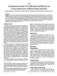
Figure 1: B eld computed in test 1.

Figure 2: B eld computed in test 2.

20

Figure 3: B eld computed in test 3.

Figure 4: B eld computed in test 4.

21

Figure 5: B eld computed in test 5.

Figure 6: B eld computed in test 6.

22