The most popular distribution for modeling count data is the ..... C. Kleiber, S. Jackman, Regression Models for Count Data in R, Journal of Statistical Software.
IJRRAS 25 (1) ● October 2015
www.arpapress.com/Volumes/Vol25Issue1/IJRRAS_25_1_01.pdf
COMPARISON COUNT REGRESSION MODELS FOR OVERDISPERSED ALGA DATA Esin Avcı1*, Sibel Alturk2, & Elif Neyran Soylu3 The University of Giresun, Science and Art Faculty, Department of Statistics, Gure Yerleskesi, 28000 Giresun, Turkey 2,3 The University of Giresun, Science and Art Faculty, Department of Biology, Gure Yerleskesi, 28000 Giresun, Turkey 1
ABSTRACT Count data become widely available in many diciplines. The most popular distribution for modeling count data is the Poisson distribution which assume equidispersion (Variance is equal to the mean). Since observed count data often exhibit over or under dispersion, Poisson models become less ideal for modeling. To deal with a wide range of dispersion levels, Quasi Poisson regresion, Negative Binomial regression and lately Conway-Maxwell-Poisson (COM-Poisson) regression used as an alternative regression models. We compare the COM-Poisson to all other regression models and illustrate its advantage and usefulness using over-dispersed alga data. Keywords: COM-Poisson regression, over-dispersed count data, Navicula cryptocephala Kutzing. 1. INTRODUCTION Count data arise in many fields, including biology, healthcare, psychology, marketing and more. When response variable is a count and the researcher is interested in how this count changes as the explanatory variable increase. Classical Poisson regression is the most well-known methods for modeling count data, but its underlying assumption of equi-dispersion (i.e., an equal mean and variance) limits its use in many real-world applications with over-or under dispersed (i.e., the variance is larger than the mean or smaller than the mean) data.This excess variation may accour incorrect inference about parameter estimates, standart errors, tests and confidence intervals. Overdispersion frequently arises for various reasons, including mechanisms that generate excessive zero counts or cencoring. As a result over-dispersed count data are common in many areas which in turn, has led to the development of statistical methodology for modeling over-dispersed data [1].For over-dispersed data, the Negative Binomial model is a popular choice [2]. Other over-dispersion models include Poisson mixtures [3], Quasi-Poisson regression and ConwayMaxwell-Poisson. Quasi-Poisson regression produces regression estimates equivalent to Poisson regression, but standart errors larger than classical Poisson regression [4].However, these models are not suitable for underdispersion. A flexiable alternative that captures both over- and under-dispersion is the Conway-Maxwell-Poisson (COM-Poisson) distribution. The COM-Poisson is a two-parameter generalization of the Poisson distribution which also includes the Bernoulli and Geometric distributions as a special ceses [5]. The COM-Poisson distribution has been used in a variety of count data application and has been extended methedologyically in various direction [6]. This article is organized as follows, Section 2 briefly describes the Poisson, Quasi-Poisson, Negative Binomial and COM-Poisson regression respectively. Section 3 presents dataset on Navicula cryptocephala Kutzing, where a sample of over-dispersed data. All mentioned regression models were applied and the results were compaired. Section 4 presents conclusion. 2. METHODS 2.1. Poisson Models Poisson regression is a special case of Generalized Linear Models (GLM) framework. The simplest distribution used for modeling count data is the Poisson distribution with probability density function 𝑓(𝑦; 𝜇) =
exp(−𝜇)𝜇 𝑦
(1)
𝑦!
The canonical link is 𝑔(𝜇) = log(𝜇) resulting in a log-linear relationship between mean and linear predictor. The variance in the Poisson model is identical to the mean, thus the dispersion is fixed at 𝜙 = 1 and the variance function is 𝑉(𝜇) = 𝜇 [7]. The mean Poisson regression can be assumed to follow a log link, 𝐸(𝑌𝑖 ) = 𝜇𝑖 = 𝑒𝑥𝑝(𝑥𝑖 ′ 𝛽), where 𝑥𝑖 denotes the vector of explanatory variables and β the vector of regression parameters. The maximum likelihood estimates can be obtained by maximizing the log likelihood.
1
IJRRAS 25 (1) ● October 2015
Avei et al. ● Comparison Count Regression Models
2.2. Quasi-Poisson Models In order to relax the Poisson assumption of equidispersion, Quasi-Poisson methods represent a potantial solution. By this way few assumptions about the dispersion for the dependent variable are required; only the relationship between the outcome mean and the explanatory variables, and between the mean and variance must be specified [8].This strategy leads to the same coefficient estimates as the standart Poisson models but inference is adjusted for overdispersion [7]. 2.3. Negative Binomial Models A second way of modeling over-dispersed count data is to assume a Negative Binomial (NB) distribution for (𝑦𝑖 |𝑥𝑖 ) which can arise as a Gamma mixture of Poisson distributions. One parameterization of its probability density function is 𝑓(𝑦; 𝜇, 𝜃) =
Γ(𝑦+𝜃)
𝜇 𝑦𝜃 𝜃
(2)
Γ(𝜃)𝑦! (𝜇+𝜃)(𝑦+𝜃)
with mean µ and shape parameter 𝜃; Γ(. ) is the Gamma function. For every fixed 𝜃 , this is another special case of 𝜇2
the GLM framework. It also has 𝜙 = 1 but with variance function 𝑉(𝜇) = 𝜇 + [7]. The mean of NB regression can 𝜃 also be assumed to follow the log link, 𝐸(𝑌𝑖 ) = 𝜇𝑖 = 𝑒𝑥𝑝(𝑥𝑖 ′ 𝛽), and the maximum likelihood estimates can be obtained by maximizing the log likelihood. 2.4. Conway-Maxwell-Poisson (COM-Poisson) Models The Conway-Maxwell-Poisson (COM-Poisson) distribution has been re-introduced bystatisticians to model count data characterized by either over- or under-dispersion [5,9,10,11]. The COM-Poisson distribution was firstintroduced in 1962 by Conway and Maxwell [12]; only in 2008 it was evaluated in the context of a GLM by Guikemaand Coffelt et al. (2008) [13], Lord et al. (2008) [10] and Sellers and Shmueli (2010) [14]. The COM-Poisson distribution is a twoparameter generalization of the Poisson distribution that is flexible enough to describe a wide range of count datadistributions [14]; since its revival, it has been further developed in several directions andapplied in multiple fields [5]. The COM-Poisson probability distribution function [5] is given by the equation: 𝜆𝑦
𝑃(𝑦; 𝜆, 𝜐) = (𝑦!)𝜐
(3)
𝑍(𝜆,𝜐)
for a random variable Y, where 𝑍(𝜆, 𝜐) = ∑∞ 𝑠=0
𝜆𝑠 (𝑠!)𝜐
, and 𝜐 ≥ 0 is a normalizing constant; 𝜐 is considered the
dispersion parameter such that 𝜐 > 1 represents under-dispersion, and 𝜐 < 1 over-dispersion. The COM-Poisson distribution includes three well-known distribution as special cases: Poisson (𝜐 = 1), Geometric (𝜐 = 0, 𝜆 < 1), and 𝜆 Bernoulli (𝜐 → ∞𝑤𝑖𝑡ℎ𝑝𝑟𝑜𝑏𝑎𝑏𝑖𝑙𝑖𝑡𝑦 )[5]. 1+𝜆
Taking a GLM approach, Sellers and Shmueli (2010) [14] proposed a COM-Poisson regression model using the link function, 𝑝
𝜂(𝐸(𝑌) = log 𝜆 = 𝑋 ′ 𝛽 = 𝛽0 + ∑𝑗=1 𝛽𝑗 𝑋𝑗
(4)
Accordingly, this function indirectly models the relationship between 𝐸(𝑌) and 𝑋 ′ 𝛽, and allows for estimating β and 𝜐 via associated normal equations. Because of the complexity of the normal equation, using 𝛽 (0) and 𝜐 (0) = 1, as starting values. These equations can thus be solved via an appropriate iterative reweighted least squares procedure (or by maximizing the liklihood function directly using an optimization program) to determine the maximum likelihood estimates, 𝛽̂ and 𝜐̂. The associated standart errors of the estimated coefficients are derived using the Fisher Information matrix [1]. 2.5. Testing for Variable Dispersion Sellers and Shmueli (2010) [14] established a hypothesis testing procedure to determine if significant data dispersion exists, thus demonstarting the need for a COM-Poisson regression model over a simple Poisson regression model; in other words, they test whether (𝜐 = 1) or otherwise [1].
2
IJRRAS 25 (1) ● October 2015
Avei et al. ● Comparison Count Regression Models
Since NB regression reduce to Poisson regression in the limit as 𝜃 → 0, The test of overdispersion in Poisson vs Negative Binom Poisson,is the test whether (𝜃 = 0) or otherwise, can be performed using Likelihood Ratio Test (LRT), 𝑇 = 2(𝑙𝑛𝐿1 − 𝑙𝑛𝐿0 ), where 𝑙𝑛𝐿1 and 𝑙𝑛𝐿0 are the models log likelihhood under their respective hypothesis. To test the null hypothesis at significance level α, the critical value of chi-square distribution with significance level 2α is used. The null hypothesis is rejected when T value exceed critical value of chi-square [15]. 2.6. Akaike Information Criteria (AIC) When several models are available, one can compare the models performance based on several likekihood measure which have been proposed in statistical literatures. One of the most popular used measure is AIC. The AIC penalized a model with larger number of parameters, and is defined as 𝐴𝐼𝐶 = −2𝑙𝑛𝐿 + 2𝑝
(5)
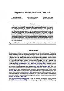
where 𝑙𝑛𝐿 denotes the fitted log likelihood and 𝑝 the number of parameters [15]. A relatively small value of AIC is favorable for the fitted model. 3. DATA ANALYSIS Navicula Cryptocephala Kutzing is one of the Epilithic algae, occur in Freshwater (more oligotrophic) habitats, including slightly humic waters. Between June 2013 and May 2014 thenumber of Navicula Cryptocephala Kutzing data are collected from four different station that located on Batlama stream. In order to model the effect of station and water temperature on the number of Navicula Cryptocephala Kutzingall the models described above applied to data set. At the end of the section, all fitted models are compared highlighting that the modelled mean function is similar but the fitted likelihood and AIC are different. The analysis are performed in R program. Respectievely, glm() function from "stats" package, glm.nb() function from "MASS" package and cmp() function from "COMPoissonReg" package are used. To obtain a first overview of the dependent variable, we are employed a histogram of the observed count frequencies. The histogram (Figure 1.) illustrates that the marjinal distribution exhibits substantial variation.
Figure 1. Frequency of Navicula Cryptocephala Kutzing A second step in the exploratory analysis is to look at pairwise bivariate displays of the dependent variable against each of the regressors bringing out the partial relationships.
3
IJRRAS 25 (1) ● October 2015
Avei et al. ● Comparison Count Regression Models
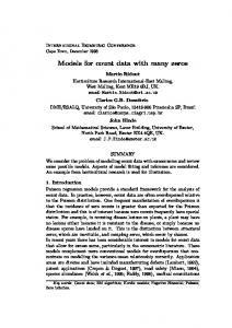
Figure 2. Box Plot of the dependent variable against station and Months All displays (Figure 2.) show that the number of Navicula Cryptocephala Kutzing increases or decreases with the regressors. The number of Navicula Cryptocephala Kutzing is slightly lower for third station compared to first station. The number of Navicula Cryptocephala Kutzing is increases with September but decreases with May. Regressing the number of Navicula Cryptocephala Kutzing on station and months (model-1) for all mentioned models. The best model is chosen using backward stepwise based on both AIC (𝐴𝐼𝐶𝑚𝑜𝑑𝑒𝑙(2) < 𝐴𝐼𝐶𝑚𝑜𝑑𝑒𝑙(1) )and p values (drop a covariate if it is not significant). Based on two test, the effect of station is not found statistically significant, we drop the station covariate, and continous with only months effect (model-2). Results of this analysis are given in table 1. Table 1 shows the parameter estimates, standart error and AIC value to chosen best model. Table 1. Parameter estimates, standart error and AIC value for models Classic Poisson Estimated Standart Coefficent Error 2.8804 0.1239 -0.0104 0.0373 -0.0604 0.0122* -
Intercept Station 1 Months Dispersion parameter 2.8543 0.0822 Intercept -0.0604 0.0122* 2 Months Dispersion parameter -219.19 Log1 liklihood 444.37 AIC -219.23 Log2 liklihood 442.45 AIC * p