Comparison of Ability Estimation and Item Selection Methods in Multidimensional Computerized Adaptive Testing Qi Diao CTB/McGraw-Hill
Mark Reckase Michigan State University Presented at the Multidimensional CAT Paper Session, June 3, 2009
Abstract The impetus of the study was the lack of guidance in the literature of multidimensional computerized adaptive testing (MCAT) in terms of which item selection and ability (θ) estimation methods to use and under what conditions. This study did a comprehensive comparison of θ estimation and item selection methods in MCAT. Two θ estimation methods included maximum likelihood and Bayesian estimation. The item selection methods can be divided into two categories, item selection methods using Fisher’s information, and item selection method with Kullback-Leibler information. When Fisher’s information was used, both D-optimality and A-optimality were investigated. The comparison was made conditioning on such factors as test length and use of priors. Simulations were based on real data from the 2005 Michigan Educational Assessment Program. As the result of the study, recommendations are made concerning which method should be used under certain conditions. It is believed that the results of the study can help future researchers in selecting θ estimation and item selection methods when conducting their own research in MCAT and assist in the construction of operational MCAT procedures.
Acknowledgment Presentation of this paper at the 2009 Conference on Computerized Adaptive Testing was supported in part with funds from GMAC®.
Copyright © 2009 by the Authors All rights reserved. Permission is granted for non-commercial use.
Citation Diao, Q., and Reckase, M. (2009). Comparison of ability estimation and item selection methods in multidimensional computerized adaptive testing. In D. J. Weiss (Ed.), Proceedings of the 2009 GMAC Conference on Computerized Adaptive Testing. Retrieved [date] from www.psych.umn.edu/psylabs/CATCentral/
Author Contact Qi Diao, CTB/McGraw-Hill, 20 Ryan Ranch Road, Monterey, CA 93940 Email:
[email protected]
Comparison of Ability Estimation and Item Selection Methods in Multidimensional Computerized Adaptive Testing Computerized adaptive testing (CAT) has been widely used in many testing programs. It is based on the principle of selecting items to match the current ability estimate of the examinees. Ample research has been done on unidimensional CAT (e.g., van der Linden & Glas 2000; Wainer 2000). However, only a few studies have been done on multidimensional adaptive testing (e.g., Segall, 1996; Veldkamp & van der Linden, 2002). There are at least three motivations for developing multidimensional computerized adaptive testing (MCAT). The first is that for many operational tests, the unidimensional models do not fit. Multidimensional response models are needed in order to satisfy the assumption of local independence. The second motivation is that for testing for diagnosis purposes, we want to extract as much information as possible, and for correlated ability dimensions information from one dimension can help measure ability in another dimension. The second motivation also leads to the third—efficiency. Because we can use information from correlated abilities, MCAT can further make the ability estimation process more efficient. For any adaptive test, five key questions need to be answered: (1) which model to use; (2) how to select the first item; (3) how to update the ability estimate after an examinee gives the response; (4) how to select the next item; and (5) how to end the test. So in order to develop any adaptive test, ability estimation and item selection methods are very fundamental. This research was targeted at investigating ability estimation and item selection in multidimensional cases. There has been some amount of research done in unidimensional CAT to investigate the properties of ability estimation and item selection methods (e.g., Weiss & McBride, 1984; van der Linden & Pashley, 2000). However, in the current literature on MCAT, most studies are done using a single ability estimation and item selection method, because they focus on other aspects of adaptive testing (e.g., Lee, Ip, & Fuh, 2008). The only study that compared different ability estimation and item selection methods is Tam (1992), but that study was completed before most of the currently used methods were developed (Segall, 1996; Veldkamp & van der Linden, 2002; Mulder & van der Linden 2010). Also, most of the research on MCAT used two-dimensional cases, but we believe that for the purpose of multidimensional tests at least three dimensions are needed. Therefore, in order to have a better understanding of MCAT, we conducted a comparative study of ability estimation and item selection methods in MCAT under different conditions. We believe the results of such study can greatly help future researchers in selecting ability estimation and item select methods when conducting their own research in MCAT and help to construct operational MCAT. The first attempt to extend unidimensional adaptive testing methods to the multidimensional case was Bloxom and Vale (1987). As mentioned above, Tam (1992) compared adaptive estimation for multidimensional tests and also developed an iterative maximum likelihood ability estimation procedure. But all studies in those times were limited by computer power, which is not a problem for the computers now. For current ability estimation methods and item selection methods, Segall (1996, 2000) applied maximum likelihood estimation and Bayesian estimation, and maximum information item selection using Fisher’s information to MCAT. Luecht (1996) examined the benefits of applying MCAT methods in a licensing/certification context. van der Linden (1999) used a minimum error variance criterion to select the next item. Another item -1-
selection method, Kullback-Leibler information was first introduced to adaptive testing by Chang & Ying (1996). Veldkamp & van der Linden (2002) further developed it into multidimensional cases. Mulder & van der Linden (2008) introduced A-optimality (minimize the trace of the inverse of the information matrix) in comparison to the traditional D-optimality (maximize the determinant of the information matrix). More detailed research on optimal design can be found in Silvey (1980). This study examined two ability estimation methods: maximum likelihood (Segall 1996, 2000) and a Bayesian method (Segall 1996, 2000). Item selection methods studied were: maximum information using Fisher’s information, and Kullback-Leibler information; these methods were compared for both D-optimality and A-optimality. The study compared the above methods under various conditions, including test length, priors used, and whether all dimensions were intentional.
Method Item Bank The item bank was simulated based on real data from the Michigan Educational Assessment Program (MEAP). Li (2006) used the data from the 2005 MEAP mathematics test for the 7th graders. This real data set included 8,562 examinees and 50 multiple-choice items. From the dimensionality analysis results of Li, this data set measured three ability dimensions: the first dimension measured ability to abstract math concepts, the second dimension measured vocabulary and operations ability, and the third dimension measured problem solving ability. Also, Li’s study showed that the test had simple structure, which means that each item loaded primarily on only one dimension. More details about the dimensional structures of the test items can be found in Reckase (2009). Based on the three-dimensional structure, Li (2006) gave all the item parameters and ability distribution of the 8,562 examinees.
Simulation Based on Li (2006)’s item parameters, 300 items were generated with 100 items primarily measuring each dimension. Because the data set was three-dimensional, 50 replications were simulated for each combination of −1, 0, 1, −1, 0, 1 and −1, 0, 1. If Bayesian methods were used, all interim ability (θ) estimates were MAP estimates and the final θ estimates were EAP estimates. Mean bias and root mean squared error (RMSE) were used as a measure of estimation accuracy. Plots of successive estimates of the locations as the test progressed were also drawn to show the speed the estimates as they converged to the true values. The compensatory twoparameter multidimensional IRT model was used to generate the item response data. One problem with maximum likelihood estimation (Segall 1996, 2000) is that it might not converge at the beginning of the test. In order to investigate that, test lengths of 20 and 50 were simulated for maximum likelihood methods. Final θ estimates were compared to the true values. In order to compare the performance of maximum likelihood and Bayesian θ estimation, both test lengths of both 20 and 50 items were generated and the simulated results were compared. For testing the impact of priors in the Bayesian method, multivariate normal distributions were used with mean 0, and variance-covariance matrix as (1) the identity matrix;( 2) diag(9), that is, all on-diagonal values were 9 and off-diagonal values were 0; and (3) the true variancecovariance matrix from the real MEAP 2005 data in Li (2006), and final θ estimates were -2-
compared. While using the maximum likelihood as the θ estimation method, with a test length of 50, tests with D-optimality and A-optimality were simulated and final θ estimates were compared. Also, while using the Bayesian θ estimation method, with the prior distribution set as standardized multivariate normal, and test lengths of 20 and 50, tests using both KullbackLeibler information and Fisher’s information were simulated and the final θ estimates were compared. Table 1 shows the simulation conditions. Table 1. List of Simulation Conditions θ Estimation Method MLE
Bayesian
Item Selection Method
Prior
D-optimality
N/A
A-optimality Bayesian Volume Decrease
N/A Mean=0, var-cov=identity matrix
Bayesian Volume Decrease
Mean=0, var-cov=diag(9)
Bayesian Volume Decrease
Mean=0, var-cov=true θ distribution
Kullback-Leibler
Mean=0, var-cov=identity matrix
Test Length 20 50 50 20 50 20 50 20 50 20 50
Results In order to investigate the non-convergence problem at the beginning of the test when maximum likelihood was used as the θ estimation method, the plot of successive estimates for one examinee with true location point (1, 1, 1) is shown in Figure 1. The initial estimate was (0, 0, 0) and the test length was 50. Figure 1 shows that at the beginning of the test, when maximum likelihood estimation was used, the estimates were not converging. They hit the ceiling we set ± 3 when the estimate was not converging. After several items, the estimate converged and became nearer and nearer to the true location point. In comparison, when Bayesian estimation methods were used, the estimate quickly converged to the true location.
-3-
Figure 1. Successive Progress Plot of Updated θ Estimates and True Location Point After Administering Each Item Initial Estimate (0, 0, 0), True Location Point (1, 1, 1), Test Length=50
One of the research questions was to compare the performance of A-optimality with Doptimality as the item selection method when maximum likelihood was used as the θ estimation method. The hypothesis was that their performance was comparable. Mean biases and RMSEs of the final estimates of both methods were compared at a test length of 50 for each dimension. Means and standard deviations of the Euclidean distance between the final estimates and true θ location points were also compared. The mean biases and RMSEs were very similar for Doptimality and A-optimality. Results showed that at the test length of 50, the two item selection methods were comparable. Figure 2 shows the comparison of mean bias and RMSE for dimension 1. For the other two dimensions, the results were similar.
-4-
Figure 2. Mean Biases and RMSEs for Maximum Likelihood as the θ Estimation Method, With D-Optimality and A-Optimality as the Item Selection Methods, Test Length =50
b. RMSE
a. Bias
The results of the means and standard deviations (SDs) of the Euclidean distance between the final estimates and true location points were measures of estimation precision over dimensions. Figure 3 shows that over all three dimensions, the estimation precision of D-optimality and Aoptimality was similar. Figure 3. Mean and SD of Euclidean Distance for Maximum Likelihood θ Estimation and Comparison of D-Optimality and A-Optimality as Item Selection Methods
a. Mean
b. SD
-5-
For the research question on the evaluation of the impact of priors on the performance of using Bayesian as the item selection method and maximizing decrement volume by Bayesian methods as the item selection method, the comparisons were made for the test length of 20 and test length of 50 and the three different variance-covariance matrices. Mean biases and RMSEs are shown in Figure 4 for test lengths of 20 and 50 items for dimension 1. The results of the other two dimensions were similar. Figure 4. Mean Biases and RMSEs for Bayesian θ Estimation and Three Types of Variance-Covariance Matrix With Test Lengths of 20 and 50 Items (Dimension 1) a. Bias, 20 Items
b. RMSE, 20 Items
c. Bias, 50 Items
d. RMSE, 50 Items
-6-
At the test length of 20 (Figure 4a), if the value of true location points on the dimension on which the biases were calculated was 0, the biases of all three priors were very close. When the true value was either 1 or −1, among the three priors the biases for the true variance-covariance matrix were the largest. The prior variance-covariance matrix as an identity matrix and diag(9) were comparable. However, overall, the biases for all three priors on all three dimensions were very small and comparable, even though the true variance-covariance matrix had the largest biases for true values away from 0. The comparison based on RMSEs (Figure 4b) showed that all three priors were comparable and there was no large difference at the test length of 20. At the test length of 50, both biases (Figure 4c) and RMSEs (Figure 4d) were very small and estimates were very accurate for all three priors. Therefore, when the test was long, the impact of the prior was small for the combination of Bayesian as the θ estimation method and maximizing volume decrement in Bayesian as the item selection method. This combination for all three priors—strong prior, relatively weak prior, and true prior—produced accurate estimates at the end of the tests. Another research question was which θ estimation method performed better, maximum likelihood or Bayesian. In order to make the comparison, the combination of maximum likelihood and D-optimality, and the combination Bayesian with maximizing volume decrement in Bayesian with an identity matrix as the prior, were compared at the test lengths of 20 and 50. The mean biases and RMSEs were compared and the results at both test lengths are shown in Figure 5 for dimension 1. The results for the other dimensions were similar. At the test length of 20, it can be seen from Figure 5a that the mean biases of maximum likelihood were much larger than those of the Bayesian method. The comparison of RMSEs (Figure 5b) also confirmed that Bayesian θ estimation outperformed maximum likelihood. Another interesting result was that when the true θ values were negative, the mean biases for the maximum likelihood method were negatively biased while for Bayesian method they were positive. When the true θ values were positive, the mean biases for the maximum likelihood method were positive and for the Bayesian method they were negative. The results in Figure 5 show that at the test length of 50, the mean biases (Figure 5c) of maximum likelihood were still larger than those of Bayesian method. RMSEs (Figure 5d) were also larger for maximum likelihood than for the Bayesian method. Therefore, even for long tests, the Bayesian θ estimation method still outperformed the maximum likelihood θ estimation method.
-7-
Figure 5. Mean Biases and RMSEs for Maximum Likelihood and Bayesian θ Estimation at Test Lengths of 20 and 50 Items (Dimension 1) a. Bias, 20 Items
b. RMSE 20 Items
c. Bias, 50 Items
d. RMSE 50 Items
The last research question was to compare the performance of volume decrement in Bayesian item selection with Fisher’s information and the performance of maximizing Kullback-Leibler information. In order to make this comparison, both methods used the prior with mean 0 and identity matrix as the variance-covariance matrix. The comparison was conditioned on test lengths. The mean biases and RMSEs for the final estimates of each dimension were calculated and Figure 6 shows the comparison test lengths of 20 and 50 items for dimension 1. The results of the other dimensions were similar. -8-
At the test length of 20 (Figure 6a), the mean biases were small for both the Bayesian Kullback-Leibler information methods, which both produced accurate final θ estimates. RMSEs were also small for both methods. From both the mean biases and RMSEs (Figure 6b), it can be seen that the Kullback-Leilber information and Bayesian methods. When the test length increased to 50, from the results of mean biases (Figure 6c) and RMSEs (Figure 6d), the precision of the two methodswere good and those two methods were comparable in terms of estimation accuracy and stability. Figure 6. Mean Biases and RMSEs for the Comparison of Kullback-Leibler and Bayesian Item Selection for Test Lengths of 20 and 50 (Dimension 1) a. Bias, 20 Items
b. RMSE, 20 Items
c. Bias, 50 Items
d. RMSE, 50 Items
-9-
Discussion This study did a comprehensive comparison of θ estimation and item selection methods in multidimensional computerized adaptive testing. Two θ estimation methods examined were maximum likelihood estimation and Bayesian estimation. The item selection methods can be divided into three categories: item selection methods associated with maximum likelihood θ estimation, maximum likelihood is not an item selection method item selection with Bayesian methods and Fisher’s information, and item selection method with Kullback-Leibler information. D-optimality (maximizing the determinant of Fisher’s information) and A-optimality (minimizing the trace of the inverse of Fisher’s information) were included for item selection methods that were associated with the maximum likelihood method. Three priors of the Bayesian method with maximizing the volume decrement using Fisher’s information were selected to measure the impact of the priors. Two different test lengths were studied—20 items and 50 items. In total, 11 combinations of θ estimation and item selection methods were simulated and compared in the study. The initial estimate for all examinees was 0 and the mean of all priors was 0. This led to a common trend for all biases. For Bayesian estimation, all biases were “inward bias.” Estimators of positive values of θi (i = 1, 2, 3) were negatively biased and the estimators of negative values were positively biased. By contrast, when maximum likelihood estimation was used, the biases were “outward bias”. Estimators of positive values of θ were positively biased and the estimators of negative values were negatively biased. From the results of mean biases and RMSEs of final θ estimates for each dimension, and means and standard deviations of Euclidean distance, maximum likelihood θ estimation did have non-convergence problems at the beginning of the test and it affected the estimation precision of the method. Plots of successive progress of updated θ estimates also supported this conclusion. Therefore, it was recommended that a longer test should be used when maximum likelihood θ estimation method was used. When Bayesian θ estimation method was used, for all the combinations of item selection methods, the comparison of test lengths of 20 and 50 showed that the precision difference was small. The final θ estimates were already stable and accurate. Therefore, if Bayesian θ estimation was used, a short test (20 or more items) could be used. The comparison of maximum likelihood and Bayesian θ estimation methods showed that Bayesian θ estimation method outperformed maximum likelihood, especially for short test length. In general, Bayesian estimation was recommended as the θ estimation method. But with Bayesian, the test designer needs to select the priors, which might not be as objective as the maximum likelihood method. Therefore, all factors need to be taken into consideration when choosing a θ estimation method. In theory, if the test length is very long, estimates for both methods should converge and the θ estimates from the two methods should be comparable. The study also evaluated the impact of priors when a Bayesian method was used. Three priors—a strong prior, a relative weak prior, and a true prior calculated from the population— were compared. When the true θ on the dimension was 0, all three priors were comparable and the mean biases were small. When the true θ was negative or positive, and opposite to the research hypothesis, the true prior did not perform as well as the other two priors. This was -10-
because the mean of multinormal distributions for all priors was 0, the priors pulled the estimates toward the mean 0. With the true prior, the force of pulling was the strongest, so the biases were the largest. But for all three priors and conditioning on both short and long test lengths, the performance of Bayesian estimation was good and the final θ estimates were stable and accurate. More studies need to be done on how to utilize the collateral information for priors to obtain better estimation with Bayesian methods. Instead of the population prior, as was used in this study, an individual prior can be used or hierarchical models could be tested to see if that can lead to better final estimation. All the priors used in study had the same values on the diagonal, respectively. This was more regular compared to cases in which variances are quite different and correlations more varied. More studies need to be done to investigate such priors to assess the impact of item selection and θ estimation methods under such conditions. Multidimensional computerized adaptive testing is a relatively new area of research. This study was a comparison of θ estimation and item selection methods to make recommendations and provide guidance in terms of what θ estimation and item selection methods to use when designing a multidimensional computerized adaptive test. The conclusions of this study were limited to the conditions of item bank, test lengths, and priors used. More θ estimation and item selection methods are being developed. So in the future, more research needs to be done to compare the new methods with the methods examined in this study. There are also other issues in multidimensional CAT, such as how to select the first item and how to end the test, which need more research.
References Birnbaum, A. (1968). Some latent trait models and their use in inferring an examinee’s ability. Lord, F. M., & Novick, M. R. (Eds.), Statistical theories of mental test scores (pp. 397-479). Addison-Wesley, Reading, MA. Bloxom, B. M., & Vale, C. D. (1987). Multidimensional adaptive testing: A procedure for sequential estimation of the posterior centroid and dispersion of theta. Paper presented at the meeting of the Psychometric Society, Montreal. Bock, R. D. & Mislevy, R. J. (1988). Adaptive EAP estimation of ability in a microcomputer environment. Applied Psychological Measurement, 6, 431-444. Chang, H.-H., & Ying, Z. (1996). A global information approach to computerized adaptive testing. Applied Psychological Measurement, 20, 213-229. Chang, H.-H., & Ying, Z. (1999). a-stratified multistage computerized adaptive testing. Applied Psychological Measurement, 23, 211-222. Hetter, R. R., & Sympson, J. B. (1997). Item-exposure in CAT-ASVAB. In W. A. Sands, J. R. Waters, & J. R. McBride (Eds.), Computerized adaptive testing: From inquiry to operation (pp. 141-144). Washington, DC: American Psychological Association. Kim, J. P. (2001). Proximity measures and cluster analyses in multidimensional item response theory. Unpublished doctoral dissertation, Michigan State University, East Lansing, MI. Lee, Y.-H, Ip, E. H., &Fuh, C.-D. (2008). A strategy for controlling item exposure in -11-
multidimensional computerized adaptive testing. Educational and Psychological Measurement, 68, 215-232. Li, T. (2006). The effect of dimensionality on vertical scaling. Unpublished doctoral dissertation, Michigan State University, East Lansing, MI. Luecht, R. M. (1996). Multidimensional computerized adaptive testing in a certification or licensure context. Applied Psychological Measurement, 20, 389-404. Lehmann, E. L., & Casella, G. (1998). Theory of point estimation. New York, NY: SpringerVerlag. McDonald, R. P. (1997) Normal ogive multidimensional model. In W.J. van der Linden & R. K. Hambleton (Eds.), Handbook of modern item response theory (pp. 258-270). New York: Springer. McDonald, R. P. (1999). Test Theory: A unified treatment. Lawrence Erlbaum Associates, Hillsdale, NJ. Mulder, J., & van der Linden, W. J. (2010). Multidimensional adaptive testing with KullbackLeibler information item selection. In W. J. van der Linden & C. A. W. Glas (Eds.), Elements of adaptive testing. New York: Springer. Owen, R. J. (1975). A Bayesian sequential procedure for quantal response in the context of adaptive mental testing. Journal of the American Statistical Association, 70, 351-356. Reckase, M. D. (1985). The difficulty of test items that measure more than one ability. Applied Psychological Measurement, 9, 401-412. Reckase, M. D. (1997). A linear logistic multidimensional model for dichotomous items response data. In W. J. van der Linden & R. K. Hambleton (Eds.), Handbook of modern item response theory (pp. 271-286). New York: Springer. Reckase, M. D. (2009). Multidimensional item response theory. New York: Springer. Segall, D. O. (1996). Multidimensional adaptive testing. Psychometrika, 61, 331-354. Segall, D. O. (2000). Principles of multidimensional adaptive testing. In W. J. van der Linden & C. A. W. Glas (Eds.), Computerized adaptive testing: Theory and practice (pp. 53-73). Boston: Kluwer. Sympson, J. B., & Hetter, R. D. (1985, October). Controlling item-exposure rates in computerized adaptive testing. In Proceedings of the 27th annual meeting of the Military Testing Association (pp. 973-977). San Diego, CA: Navy Personnel Research and Development Center. Tam, S. S. (1992). A comparison of methods for adaptive estimation of a multidimensional trait. Unpublished doctoral dissertation, Columbia University, New York City, NY. van der Linden, W. J. (2000). Constrained adaptive testing with shadow tests. In W. J. van der Linden & C. A. W. Glas (Eds.), Computerized adaptive testing: Theory and practice (pp. 27-52). Boston: Kluwer. van der Linden, W. J., & Glas, C. A. W (Eds) (2000). Computerized adaptive testing: Theory and practice. Boston: Kluwer. van der Linden, W. J., & Veldkamp, B. P. (2004). Constraining item exposure in computerized -12-
adaptive testing with shadow tests. Journal of Educational and Behavioral Statistics, 29, 273291. van der Linden, W. J., & Veldkamp, B. P. (2007). Conditional item-exposure control in adaptive testing using item-ineligibility probabilities. Journal of Educational and Behavioral Statistics, 32, 398-418. Veldkamp, B. P., & van der Linden, W. J. (2002). Multidimensional adaptive testing with constraints on test content. Psychometrika, 67, 575-588. Wainer, Howard (2000). Computerized adaptive testing: A primer, 2nd Ed. Mahwah, NJ: Lawrence Erlbaum Association.
-13-