The methods are applied on a number of significant chemical engineering ... of the different methods when solving problems of varying complexity and size.
Computers chem. Engng Vol.20, Suppl.,pp. $333-$338, 1996
Pergamon
S0098-1354(96)00066-X
Copyright© 1996ElsevierScienceLtd Printed in GreatBritain. All rightsreserved 0098-1354•96 $15.00+0.00
C O M P A R I S O N OF D I F F E R E N T M I N L P M E T H O D S A P P L I E D O N CERTAIN CHEMICAL ENGINEERING PROBLEMS HANS SKRIFVARS, IIRO HARJUNKOSKI, TAPIO WESTERLUND ZDRAVKO KRAVANJA* and RAY PORN /~bo Akademi University, Process Design Laboratory Biskopsgatan 8, FIN - 20500/~bo, Finland *University of Maribor, Faculty of Chemistry and Chemical Engineering Smetanova 17, SLO - 62000 Maribor, Slovenia
A b s t r a c t - In this paper a comparison of some of the methods available for solving mixed integer non-linear programming (MINLP) problems is presented. Since some methods solve both a mixed integer linear programming (MILP) master problem and non-linear programming (NLP) subproblems during the iterations, while others only solve MILP master problems, a comparison of the computer resources needed for the optimization is presented. The methods are applied on a number of significant chemical engineering problems involving both MINLP problems (with a variety in the degree of discreteness and complexity) and some strict integer non-linear programming (INLP) problems. Prom the results, it is to be seen that a comparison of only the number of iterations needed in the optimization, doesn't allways measure the actual required resources of the optimization. Keywords - Mathematical Programming, Optimization, MINLP, INLP, MILP, Process Synthesis, Process Integration, Design Optimization. INTRODUCTION In recent decades, a number of methods for solving mixed integer non-linear programming (MINLP) problems have been presented and developed. This development has lead to the ability to extend process optimization to include the optimization of problem structure, process synthesis and the topology of processes, almost entirely, beyond the parametrical optimization of merely the continuous variables in processes. An increasing number of papers presenting examples of MINLP problems and solutions have been published in the chemical engineering literature during recent years. However, only a few papers present comparisons of the different methods when solving problems of varying complexity and size. MINLP problems containing mainly continuous or containing mainly discrete variables, but otherwise of the same size, are typically of very different complexity. Thus, knowing the type of the MINLP problem is also of importance. In the following sections certain numerical examples are considered. The first examples are taken from a paper by Duran and Grossmann (1986). In these problems the solutions with the Outer Approximation (OA) (Duran and Grossmann, 1986), the Generalized Benders Decomposition (GBD) (Geoffrion, 1972) and the Extended Cutting Plane (ECP) (Westerlund and Pettersson, 1995) are compared. The problems are convex MINLP problems of minor size, and only the number of iterations are compared. In the next section of examples, the OA and ECP methods are compared when solving some large convex MINLP problems appearing in simultaneous model structure and parameter estimation problems in FTIR spectroscopy. In these problems, the comparison is made both with regard to the number of iterations and the CPU-time used. In the final section of examples some large convex INLP problems, arising from trim loss problems connected to the paper converting industry, are solved. Since the OA, GBD and ECP methods are identical solution methods for convex strict integer non-linear programming (INLP) problems, only solutions with the ECP method are given.
PROCESS SYNTHESIS PROBLEMS In (Duran and Grossmann, 1986) four numerical examples of process synthesis problems formulated as MINLP problems are presented. Examples 1, 2 and 3 consider a simultaneous structural and parametrical optimization of a process flow-sheet, where binary variables are used to describe the existence of process units, and the continuous variables represent dimensional and operational parameters, such as flow rates and vessel volumes in the process. The fourth example is a formulation of the problem of determining the optimal positioning of a new product in a multi-attribute space. The first three examples present a moderate degree of complexity, in the form of the number of discrete variables and non-linear constraints and are quite easily and quickly solved by the algorithms. In the fourth, the number of discrete variables is five times the number of continuous variables, and the number of nonlinear constraints is also five times the number of $333
S334
European Symposiumon Computer Aided Process Engineering--6. Part A
linear constraints, so this problem could be considered as a more difficult one to optimize. The total number of variables and constraints in this example is greater than in the other examples, which also adds to the complexity of the problem. The number of continuous and discrete variables, as well as the number of linear and non-linear constraints for these problems, are given in Table 1. Example Variables Constraints GBD # OA # ECP number Cont. I Int. Linear Non-lin. Iterations Iterations Iterations 1 3 3 4 3 4 2 4 2 6 5 11 4 8 3 6 3 9 8 19 5 10 4 8 4 5 25 5 25 35* 6 6 # iteration numbers as reported in (Duran and Grossmann,1986) * up to 35 iterations reported, no optimal solution found Table 1. Required resources in the optimizations When analyzing the results given in Table 1 an interesting observation can be made. The OA generally uses fewer iterations than both the GBD and the ECP methods, and the ECP method generally uses fewer iterations than the GBD method in these examples. In Example 4, the OA and the ECP use the same number of iterations. It should, however, be observed that no NLP sub-problems are solved in the ECP iterations. Thus the required computer resources cannot be directly compared based on the number of iterations. The computation time in these problems is of the order of tenths of a CPU-second (on a DEC 3000 m900 AXP), therefore no considerable conclusions regarding the efficiency of the solution methods should be drawn from only the number of iterations in these examples. A FTIR PARAMETER ESTIMATION PROBLEM This example is based on a problem in quantitative FTIR-spectroscopy. A more detailed presentation of the problem can be found in (Brink and Westerlund, 1995). Infra-red spectroscopy is based on the principle that most molecules absorb electro-magnetic radiation in a unique pattern. In a multicomponent system, the absorbance Atot at wave number u can be written as the sum of the individual absorbances a~ of each component with a concentration ci N
(1)
Ato~ (u) = Z ai (v) bc, i----1
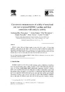
The optical path length b is usually held constant during the calibration and prediction stages, and the two first terms on the right hand side can thus be expressed as a single constant. A spectrum for a multicomponent system is usually recorded over thousands of wave numbers. In our case, all spectra are recorded for wave numbers from 875 cm -1 to 2200 cm -1.
0.50 0.45 0.40
(D
0.35
q;
0.30 ~ 0,25
X:~
0.20 ~0 0.15
O.lo 0.05 0
o
_j
o
Figure 1. FTIR spectra for 35 different concentration combinations In order to solve the opposite problem of estimating the concentrations from individual spectra, we can use a linear model of the form c = Pa (2) which relates the absorbances to the concentrations. Here e is the concentration vector, P a parameter matrix and a is a vector containing the spectra. The main difficulty when estimating the parameters in the model from spectra and corresponding concentration data is that only a restricted number of wave numbers can be included due to the lack of degrees of freedom in multiple regression analysis. One way to overcome
European Symposium on Computer Aided Process Engineering----6.Part A
$335
this problem is to use an information criterion to determine both the model structure (i.e. which pazameters in (2) should be equal to zero and which should not) and to estimate the model parameters. One such criterion that allows this to be done is the Akaike Information Criterion (AIC) (Akaike, 1974) . The AIC is given by AIC = - 2 1 n L + 2p (3) where L is the likelihood function and p is the number of parameters in the model. By combining AIC and the likelihood function as presented in (Brink and Westerlund, 1994), we obtain a MINLP problem of the form min
Z =
eWR-lek + 2.
/~i
(4)
subject to: 0i - 0i . . . . •/3i < 0
, i = 1,...,Ptot
(5)
--Oi "q- Oi,min " / ~ i ~ 0 , i = 1 , . . . , Ptot (6) /~ = vec (P), where vec 0 is the row string operator. ~i are binary variables describing the existence of the corresponding parameter/9i, ek are the residuals of the concentration vector e for observation k, and P~ is the corresponding residual covaxiance matrix. For a given residual covaxiance matrix, the problem is a convex MINLP problem. In the following, some examples of the above formulation are considered. In all of the examples an identity matrix has been used as the covaxiance matrix. In the first example, 8 spectra (i.e.corresponding to 8 different combinations of the concentrations of the components), each with absorbances at 10 wave numbers, are used. The second and third examples both use the 35 different spectra in Figure 1, with absorbances at 100 and 200 wave numbers, respectively. The problems are solved with both the Outer Approximation (OA) and the Extended Cutting Plane (ECP) methods. Since these problems are much larger than the previous examples, results for the required resources in the form of both the number of iterations and the CPU-time used (on a DEC 3000 mP00 AXP) are presented in Table 2 below. The values Omin = 0 and Oma== 1000 were used in the optimizations. Example Variables Constraints OA ECP number Cont. 1 Int. Lineax'Non-lin. 1 Iter. CPU2(s).9 Iter. CPU (s) 1 31 30 60 1 21 64 21.9 2 301 300 600 1 27 214.5 57 158.4 3 601 600 1200 1 37 3539.2 81 6125.7 I including
the objective
function
Z
Table 2. Required resources in the optimizations From the table above, it can be seen that the Outer Approximation method, as in the previous examples, generally needs fewer iterations than the Extended Cutting Plane method for convergence. However, since every iteration in OA solves both a MILP master problem and a corresponding NLP sub-problem, one iteration in the OA method requires more computer resources than in the ECP method. It is thus not obvious which method uses less CPU-time totally. As can be seen in Table 2, we find that the OA method uses less CPU-time in Examples 1 and 3 while the ECP method uses less CPU-time in example 2. The upper and lower bounds for the OA and the ECP methods when solving Example 2, axe given in Figure 2, versus the number of iterations and versus the CPU-times used. OA & ECP OA & EGP 100 ab6orbances,covadancematrix#1 (=I) 200
'l^1
I I
100 absodoances,covariancematrix #1 (=I) . . . .
200
I 150
=e 150
[,oo
L
e.
~ 1oo
E~P 0 .........
o
OA
:,
,o
2o
0
'so
'4o
Iteration Number
so
~
ro
I
o
so
loo
~ I
1~o
CPU time (s)
Figure 2. Convergence of lower and upper bounds for OA and ECP in FTI'R Example 2
200
S336
European Symposium on Computer Aided Process Engineering--6. Part A
As can be seen in Figure 2, the convergence in iterations is opposite the CPU-time for the methods. From the figure it can also be found that the upper and lower bounds are much tighter for the ECP method compared to the bounds for the OA method, already after a moderate amount of CPU-time, while the opposite holds for the iterations. For Examples 1 and 3 both the numbers of iterations and the total CPU-time was found to be shorter for the OA method compared to the ECP method. But, when a similar figure to Figure 2 was plotted, it was found that the transient period for convergence (in CPU-time) was almost identical for both methods in Example 3. The transient convergence was found to be faster for the OA method in the first example. T R I M LOSS P R O B L E M Trim loss problems are commonly encountered in the paper converting industry. The problem is to cut wider raw-paper rolls into narrower product paper rolls, such that the loss of paper and cutting time are minimized subject to physical constraints in the cutting, and such that the required number of product paper rolls is produced. The required number of product paper rolls of each type i is given by the number iV/ and the corresponding widths are/3/. The width of the raw paper roll is given by Bm~z. The cutting patterns to be solved can be defined by the variables nq, corresponding to the number of product paper rolls of type i at the cutting pattern j , and mj is the multiple of the cutting pattern j. A physical restriction in each cutting pattern is that the number of product rolls should not exceed Nma~. In order to define the existence of a cutting pattern, the binary variables yj are defined. Minimizing the total cost of raw-paper and costs of the cutting patterns (knife changes) results in a INLP problem of the following form
min
m~ ,Yi,n~J
{~(cffnj+Cjyj)}
(7)
j----1
Subject to: I
Z Binij - Bma~: