COMPUTER VISION AND IMAGE UNDERSTANDING
Vol. 69, No. 1, January, pp. 38–54, 1998 ARTICLE NO. IV960587
Comparison of Edge Detectors A Methodology and Initial Study∗ Mike Heath,† Sudeep Sarkar,† Thomas Sanocki,‡ and Kevin Bowyer† †Computer Science & Engineering, ‡Department of Psychology, University of South Florida, Tampa, Florida 33620 E-mail:
[email protected],
[email protected],
[email protected],
[email protected] Received January 30, 1996; accepted December 3, 1996
between ratings for fixed versus adapted parameters? 2. Is there interaction between fixed versus adaptive parameter values and the edge detectors? 3. For fixed parameters, are there differences in ratings between edge detectors? 4. For fixed parameters, is there interaction between the detector and the image? 5. For adapted parameters, is there a difference in the ratings between edge detectors? 6. For adapted parameters, are there interactions between edge detectors and images? D. Summary. VI. Discussion and conclusion. A. Observations. B. Experimental concerns.
Because of the difficulty of obtaining ground truth for real images, the traditional technique for comparing low-level vision algorithms is to present image results, side by side, and to let the reader subjectively judge the quality. This is not a scientifically satisfactory strategy. However, human rating experiments can be done in a more rigorous manner to provide useful quantitative conclusions. We present a paradigm based on experimental psychology and statistics, in which humans rate the output of low level vision algorithms. We demonstrate the proposed experimental strategy by comparing four well-known edge detectors: Canny, Nalwa–Binford, Sarkar–Boyer, and Sobel. We answer the following questions: Is there a statistically significant difference in edge detector outputs as perceived by humans when considering an object recognition task? Do the edge detection results of an operator vary significantly with the choice of its parameters? For each detector, is it possible to choose a single set of optimal parameters for all the images without significantly affecting the edge output quality? Does an edge detector produce edges of the same quality for all images, or does the edge quality vary with the image? °c 1998 Academic Press Key Words: edge detection; low-level processing; segmentation; performance evaluation.
I. INTRODUCTION What is more interesting is that we are willing to develop one more edge detector, but we do not want to develop objective and quantitative methods to evaluate the performance of an edge detector. About three decades of research on edge detection has produced N edge detectors without a solid basis to evaluate the performance. In most disciplines, researchers evaluate the performance of a technique by a controlled set of experiments and specify the performance in clear objective terms. In edge detection, practically no efforts were even made to define objective measures. We still evaluate the performance of an edge detector by looking at the results. (Ramesh Jain and Tom Binford, 1991)
The ubiquitous interest in edge detection stems from the assumption that object boundaries manifest as intensity changes. The front end of most vision systems consists of an edge detection module. Quantitative performance comparison of these low level vision modules requires ground truth. In fact, Hoover et al. [2] at USF have recently conducted such a comparison study based on manually constructed ground truth for range segmentation tasks. However, manually constructing ground truth for real intensity images is problematic. Even the definition of an intensity edge is debatable. Should one consider just step edges? What should be the ideal profile of a step edge? Where would the edge location be marked for a gradually changing edge? Hence, we believe that in the near future creating ground truth of realistic intensity images is a practical impossibility. The difficulties involved in obtaining ground truth for real images are so great that, as evidenced by the prior work data summarized in Table 1, researchers simply do not conduct quantitative evaluations of edge detectors using real images. (Table 1 lists contributions to the problem of edge detection recently published
CONTENTS I. Introduction. II. Related work. III. Methods. A. Edge detectors. B. Images. C. ANOVA. IV. Experiment #1: Edge detector parameter settings. A. Edge detector parameter settings. B. Images. C. Judges for the rating task. D. Rating task. E. Results. 1. Are the ratings of the judges consistent? 2. Do the ratings of an edge detector vary with the image? 3. Does the rating of an edge detector rating vary with its parameter? 4. Is there interaction between the chosen edge detector parameter value and the image? F. Summary. V. Experiment #2: Comparison rating of edge detectors. A. Judges for the rating task. B. Rating task. C. Results. 1. Is there a statistically significant difference
∗ This work is supported by Air Force Office of Scientific Research Grant F49620-92-J-0223 and National Science Foundation Grants CDA-9424214, DBS-9213246, and IRI-9501932. 38 1077-3142/98 $25.00 c 1998 by Academic Press Copyright ° All rights of reproduction in any form reserved.
39
EDGE DETECTORS: METHODS AND STUDY
TABLE 1 Edge Detection Algorithms in PAMI (Jan. 93–June 95), SMC (Jan. 93–Aug. 95), R&A (April 94–June 95), CVGIP (Jan. 90–July 95), IJCV (Jan. 90, Dec. 94), PR (Jan. 93–July 95)
Source [3] (PAMI, 1995) [4] (PAMI, 1994) [5] (PAMI, 1993)
Nature of the algorithm
Performance presented on
Real image ground truth
[6] (PAMI, 1993) [7] (SMC, 1995) [8] (SMC, 1994) [9] (CVGIP, 1994)
Covariance models Expansion matching Dispersion of gradient direction Regularization Surface fitting Neural networks Voting based
[10] (CVGIP, 1994) [11] (CVGIP, 1992) [12] (CVGIP, 1991) [13] (CVGIP, 1991) [14] (CVGIP, 1991) [15] (IJCV, 1994) [16] (IJCV, 1994) [17] (IJCV, 1993)
Linear filtering Maximum likelihood Linear filtering Linear filtering Derivative based Linear filter Linear filter Analog network
2 real 2 synth 2 real 3 real 3 range 2 synth 1 real, 1 synth 1 synth 3 real, 1 synth 2 real 1 real 1 synth, 2 real 1 synth 2 real
[18] (PR, 1995) [19] (PR, 1995)
Statistical Search
4 real 1 synth, 3 real
0 0 0 0 0 0 0 Reconstructed image as ground 0 0
[20] (PR, 1995) [21] (PR, 1994) [22] (PR, 1994) [23] (PR, 1994) [24] (Pr, 1994)
Filtering Neural nets Genetic opt. Co-occurrence Statistical
4 real 1 synth, 1 real 1 synth, 1 real 4 synth, 2 real 1 synth, 1 real
0 0 0 0 0
[25] (PR, 1993) [26] (PR, 1993) [27] (PR, 1993)
Local masks Filtering Statistical
2 synth, 2 real 1 real 3 real
0 0 0
Algorithms compared
3 real 1 real 1 real
0 0 0
None Canny Sobel
0 0 0 0
LoG, Canny Sobel, Haralick None Canny
LoG Rosenfeld & Thurston LoG, Canny Deriche None None None Log Canny, LoG Canny, LoG, Ashkar & Modestino None Canny Simulated anneal local search Canny, LoG, Jain’s stochastic Sobel, DoG, Haralick, Anisotropic diffusion Other hierarchical 0 Nalwa, DoG
Note. The number of images is counted from the images presented in the paper. Ground truth is counted as objective specification of correct edge pixels. The last column lists the edge algorithms considered in the comparison.
in major journals.) Quantitative evaluation, when done at all, is done on synthetic images. However, most researchers do not regard results on synthetic images as convincing and still desire to see results on real images. Another possible strategy would be to measure the performance enhancement of a complete general vision system with different edge detectors. Unfortunately, there is no such competent computer vision system. Thus, it has become an accepted practice to compare edge detectors by presenting visual results side-by-side for the reader’s subjective evaluation. That is, we resort to asking the only known object recognition system with proven competence—the human. But this practice raises many questions. How variable is the subjective judgement about an edge detector across images? How well do different people agree in their subjective judgments of an image? To what extent are the conclusions affected by choice of images?
The purpose of this paper is to describe a new (to computer vision) experimental framework which allows us to make quantitative comparisons using subjective ratings made by people. This approach avoids the issue of pixel-level ground truth. As a result, it does not allow us to make statements about the frequency of false positive and false negative errors at the pixel level. Instead, using experimental design and statistical techniques borrowed from psychology, we make statements about whether the outputs of one edge detector are rated statistically significantly higher than the outputs of another. We believe that edge characterization has to be done in the context of a visual task. The edge evaluation strategy depends on what we want to do with the edges. In the proposed framework, the edge ratings are done in the context of object recognition. The edges are rated by human experts according to whether all of the edge information relevant for recognizing an object is
40
HEATH ET AL.
present, without distracting edges. The experts in our study are students with extensive experience in dealing with images on the computer. The paper is organized as follows. Related work is discussed in the next section. The edge detectors and the image set are discussed in Section III. The comparison was conducted in two stages. Every edge detector has parameters whose values need to be set. In the first stage, discussed in Section IV, we conducted experiments to choose these parameter values. Then the outputs of the edge detectors were compared in the second set of experiments, described in Section V. We discuss the results and conclude with Section VI. II. RELATED WORK Recent work in the design of edge detectors is summarized in Table 1. Our work deals not with the design of an edge detector, but rather the methodology for comparing edge detectors. One of the earliest comparisons was done by Abdou and Pratt [28]. This was followed by work by Fram and Deutsch [29], Peli and Malah [30], and more recently, Ramesh and Haralick [31]. The emphasis in this line of work has been to characterize the edge detector based on local signal considerations. The typical quantitative measures have been the probability of false alarms, probability of missed edges, errors of estimation in the edge angle, localization errors, and the tolerance to distorted edges, corners, and junctions. While these “signal based” approaches are valuable and have their place, we believe that local, signal based measures fail to capture the globally coherent nature of perception. In this view, it is not surprising that the field contains many papers describing “optimal” edge detectors, all of whose performance leaves something to be desired. This would be the natural result of using criteria for optimality which do not adequately characterize the real-world problem. (And as commented by Haralick and Shapiro [32], “all evaluation metrics... leave something to be desired.”) We are not proposing optimality criteria which appropriately capture the nonlocal and Gestalt-like nature of object recognition. However, techniques do exist to use subjective ratings by human judges in an objective and quantitative manner. This approach offers itself as a nice complement to signal-based quantitative measures. This approach is also compatible with recent suggestions by other researchers: Objective evaluation of an early vision algorithm is difficult without specifying the purpose of a total system which includes the algorithm. One possible way is to compare the performance of an algorithm with that of human vision. (Shirai, 1994) Although it would be nice to have a quantitative evaluation of performance given by an analytical expression, or more visually by means of a table or graph, we must remember that the final evaluator is man and that his subjective criteria depend on his practical requirements. In order to do this, a better presentation of the output may help to make judgments about the obtained results (partial and final); image visualization in a controlled environment with real time presentation greatly facilitates the observers’s evaluation. (Cinque, Guerra, and Levialdi, 1994)
We agree with the quote above that ratings of a computer vision algorithm have to be made in the context of a visual task [33]. So far, edge detection modules have been designed and evaluated in isolation, except for the recent work by Ramesh and Haralick [31]. The evaluation paradigm in this paper is goal oriented; in particular, we consider edge detection in the context of object recognition. The human judges rate the edge detectors based on how well they capture the salient features of real objects. We also firmly believe that evaluation should be done using real images. As Zhou, Venkateshwar, and Chellapa [35] note, “any conclusions based on these comparisons of synthetic images have limited value. The reason is that there is no simple extrapolation of conclusions based on synthetic images to real images!” The use of human judges to rate image outputs must be approached systematically. Experiments must be designed and conducted carefully, and results must be interpreted with the appropriate statistical tools. The use of statistical analysis in vision system performance characterization has been rare. The only prior work in the area that we are aware of is that of Nair et al. [36], who used statistical ranking procedures to compare neural network-based object recognition systems. In a related work, in 1975 Fram and Deutsch [29] used human subjects to judge the discriminability of certain synthetic edge signatures. These results were then compared with the edge detectors available at that time. The focus was on human versus machine performance rather than using human ratings to compare different edge detectors.
III. METHODS A. Edge Detectors Four different edge detectors were selected for comparison. These are (1) the well-known Canny edge detector [37], (2) the traditional Sobel edge detector, supplemented with hysteresis thresholding as used in the Canny, (3) the Nalwa–Binford edge detector [38], and (4) the Sarkar–Boyer edge detector [12]. The Sobel is the baseline historical “standard” and is still frequently used in published research today. The Canny is a modern “standard,” in the sense that papers describing new edge detectors often compare the results to those of the Canny, as evidenced in Table 1. The Nalwa–Binford edge detector was chosen to represent the “surface fitting” approach to edge detection. The Sarkar–Boyer edge detector was chosen to represent the current state of the art in the “zero crossing” approach. Each of the detectors, other than the Sobel, has been described in a publication in a top journal. The implementation of the Sobel edge detector was written by us. The implementation of the Canny edge detector originally came from the University of Michigan and was incrementally modified by us. The implementations of the Nalwa–Binford and Sarkar–Boyer edge detectors were obtained from the original authors. (We do not attempt to explain
EDGE DETECTORS: METHODS AND STUDY
the technical details underlying each of the edge detectors here. The interested reader may consult the original publications [12, 37, 38].) B. Images Figure 1 shows the eight images that were used in this experiment. We chose the images to represent a wide variety of
41
objects and contexts. Each image contains a single complete object in the central portion of the image, photographed from an intuitively typical orientation, pretty much as initially encountered in its natural setting. The objects were choosen so that they are readily recognized by humans at the entry level, the first category level that comes to mind when viewing an object. To verify this we ran experiments in which images were shown for 1 s and subjects attempted to
FIG. 1. The eight images used in the experiments.
42
HEATH ET AL.
FIG. 1—Continued
identify them. The percentage of subjects providing either the correct name for the object or a synonym averaged 98.5% across the images, indicating that the objects are easily and readily recognizable by humans. The original color negatives were digitized and converted to grayscale intensity images. The contrast and brightness of the images were changed to improve their quality on slides and to make them suitable for the psychological experiment of the previous paragraph. The images were then downsampled to 512 by 512, and some were cropped so there would be only one
complete object located in the center of the image. This results in some variation in the final image size. C. ANOVA In our analysis of the experimental data we used the analysis of variance (ANOVA) technique to separate the dependencies among the variables and to ascertain the statistical significance of observed differences. For the theory behind ANOVA analysis and a full development of the approach, we refer the reader to a
EDGE DETECTORS: METHODS AND STUDY
relevant textbook (for example, [39, 40]). Here, we give only a brief sketch of how the approach is applied. The subject’s ratings of the edge images are a function of the images, edge detectors, their interaction, and random error (or “noise”). Considering the overall variance of the subject ratings gives us a global idea of the variation, but it does not tell us how the ratings (the dependent variables) vary with the individual independent parameters and their interaction. In other words the overall variance does not let us pinpoint the source of the variance to the individual independent variables. However, ANOVA allows us to accomplish this in an elegant manner. In essence, the ANOVA involves a linear regression model in which subject’s ratings are the dependent variable and the independent variables are detectors, images, and their interaction (combined effects). ANOVA separates and compares variation due to the independent variables to variation due to error. In our case, the error is the random individual differences among raters (or experimental “noise”). For example, consider that a set of Ne edge detectors are run on each of a set of Ni images and that each edge detection is rated by N j judges. The total variance would be the sum of differences of each of the Ne × Ni × N j individual ratings from the overall mean rating. The ANOVA procedure divides this total variance into four portions: one due to the edge detector, one due to the image, one due to the interaction of detector and image, and one due to “error” (random variations between raters). The interaction of detector and image is the unique effect of a combination of detector and image. It is equal to the variance leftover after subtracting the individual, additive effects of detector and image. By comparing the variance due to an independent variable to the error variance, it is possible to estimate how likely it is for the variance due to the independent variable to have arisen by chance. If the variance of the independent variable is much larger than the error variance, then it is unlikely to be due to chance and we conclude that the effect of the independent variable is probably real or statistically significant. It is also possible to compare the relative magnitude of the variances for the different independent variables and judge which independent variable has more effect on the rating, using an effect-size analysis. This analysis uses the sources of variance in the ANOVA to determine the sizes of the effects of (amounts of variance due to) images, detectors, and their interaction, relative to the amount of error. This ratio is termed omega squared [39]. It may also be noted that regression is notorious for its lack of robustness due to outliers which in our case occurs when the ratings of a few judges are not “consistent” with others. As discussed later, we explicitly check for this rater consistency to check for the presence of outlier ratings. We have not found outliers to be a problem in our experiments. IV. EXPERIMENT #1: EDGE DETECTOR PARAMETER SETTINGS ... all the edge detectors referred to above need one or two thresholds to be preset; we have observed in our experiments (We are certain that previous
43
researchers have too) that results vary considerably based on the thresholds used.... (Zhou, Venkateshwar, and Chellappa, 1989)
This first experiment is aimed at determining whether (1) it is sufficient to use a fixed set of parameter values for a given edge detector across all of our test images, or (2) it is necessary to allow the parameter settings to vary between images. If the conclusion is that a fixed parameter set is sufficient, then the experiment should identify a parameter set for each edge detector. If the conclusion is that the parameter set should vary with image, then the experiment should identify an appropriate parameter set (for each edge detector) for each of the test images. A. Edge Detector Parameter Settings Each edge detector has some parameters which must be set to appropriate values. For a comparison of edge detectors to be worthwhile, the set of parameter values used in each detector must be “tweaked” equally well. For each detector, we identified the most relevant parameters to be considered in tuning, based on suggestions in the original papers describing the edge detectors and on our own experimentation with them. For the implementation of the Sobel evaluated here, the two parameters considered in tuning are just (1) the value of the low edge strength threshold for hysteresis and (2) the value of the high threshold for hysteresis. For the Canny, the three parameters considered in tuning are (1) the low hysteresis threshold, (2) the high hysteresis threshold, and (3) the σ of a Gaussian which controls the amount of smoothing. For the Nalwa–Binford detector, the two parameters considered in tuning are (1) a blurring parameter which reflects the degree of edge blur within the fixed (five pixel) operator window and (2) the scaled edge contrast threshold. The latter contrast threshold (as in the source code) is actually twice the step edge height in gray levels. For the Sarkar–Boyer detector, the parameters considered in tuning are (1) the scale of the operator and (2) the edge contrast threshold. Note that the edge contrast thresholds in the Nalwa–Binford and Sarkar–Boyer detectors are not necessarily directly comparable, since each filter may scale the image values differently. The choice of any edge detector parameter is crucial. Because of the high combinatorics of the experimental protocol (8 to 16 judges for 8 images over edge parameter combinations), we have to restrict the edge parameters to be from a small set of values. It is well known that the choice of the edge detector parameter is dependent on the image resolution and the size of the object of interest. It is difficult to generalize a choice across all possible images. For example, the edges with a σ of one for the Canny operator on a 512 × 512 image will differ from that on the same image subsampled to 256 × 256. Hence, it is imperative to experiment with our present set of images. For each edge detector, the plausible meaningful range of each parameter was determined by consulting the original paper and experimenting with the implementation. From two to four settings of each parameter value were chosen to coarsely sample the plausible meaningful range. This resulted in from 6 to 12 combinations of parameter settings for each edge detector. Table 2 summarizes the
44
HEATH ET AL.
TABLE 2 Combinations of Parameter Settings for the Edge Detectors Canny Low hysteresis threshold
High hysteresis threshold
σ
70%, 85%
0.8, 1.4, 2.0 pixels
30%, 50%
Nalwa–Binford Blurring parameter
Minimum edge contrast (scaled)
0.25, 0.6, 0.95
30, 45, 60 gray levels Sarkar–Boyer
Scale of operator
Minimum edge contrast (scaled)
0.4, 0.8, 1.2
10, 25, 40 Sobel
Low hysteresis threshold
High hysteresis threshold
30%, 50%
70%, 80%, 90%
particular combinations of parameter values evaluated for each detector. B. Images Each of the eight images (Fig. 1) was edge detected using each set of parameter values for each detector. Thus there were 6 edge detected versions of each image for the Sobel, 12 edge detected versions of each image for the Canny, 9 edge detected versions of each image for the Nalwa–Binford, and 9 edge detected versions of each image for the Sarkar–Boyer. Printed versions of the original images and the edge detected versions of each image became the input to a rating task.
for the Canny it was 96 (8 × 12). The task was to rate the edge detected versions on a scale of 1 (low) to 7 (high). A rating of 1 was defined as “edges seem to be without coherent organization into an object.” A rating of 7 was defined as “all relevant edge information for recognizing an object with no distracting edges.” A sample rating sheet appears in the Appendix. The different sittings lasted in the range of 20 to 40 min, depending on the edge detector and with some variation between judges. The judges did not know which edge detector was being rated in a particular session. E. Results The raw data can be conceptualized as a large multidimensional data set organized as (eight judges) × (eight images) × (four edge detectors) × (six to twelve parameter sets). Recall that the different edge detectors were rated in different sittings on different days. Thus, this experimental design is not ideal for making comparisons of one edge detector against another. In this experiment we consider each edge detector individually and compare the ratings of its various parameter settings. 1. Are the ratings of the judges consistent? If the judges’ ratings are inconsistent, then further analysis of the data is problematic. Thus, the issue of consistency between the judges’ ratings is considered first. The tool for analyzing consistency between judges is the intraclass correlation coefficient (ICC). There are a number of possible forms of the ICC and it is important to select the appropriate one. In this experiment, the judges rate edge images with different parameter settings of an edge detector, and the goal is to determine the best parameter setting. So the ICC should reflect the consistency in the judges’ mean rating of a particular parameter setting’s edge image relative to the overall mean of the edge images for that edge detector. Following Shrout and Fleiss [41], the appropriate ICC is “ICC(3, k),” defined as ICC(3, k) =
C. Judges for the Rating Task Eight subjects acted as “judges” for the rating task. The judges were all undergraduate majors in computer science or computer engineering. They performed the rating task as part of their participation in an NSF-funded “Research Experiences for Undergraduates” program. They had already had some lecture and reading material on edge detection and object recognition before performing the rating task. D. Rating Task The rating task was performed in multiple “sittings” across different days. There was one “sitting” for each edge detector. On a given sitting, each of the eight judges received a stack of printed pages containing the eight original images and the corresponding edge-detected versions for one edge detector. For the Sobel, the total number of edge images for each judge was 48 (8 × 6); for the Nalwa–Binford and Sarkar–Boyer it was 72 (8 × 9); and
BMS − EMS , BMS
where BMS is the mean square value of the rating between judges and EMS is the total mean square error as defined below. Let the rating of the ith judge on the jth edge image be denoted by X i j and the total number of judges and images be a and b, respectively.P The mean of the ratings of ith judge is denoted by X¯ i. = (1/b) j X i j . The mean of the ratings for the jth P image P is X¯ . j = (1/a) i X i j . And the overall mean is X¯ = (1/ab) i j X i j . Then, BMS =
b X ¯ ( X i. − X¯ )2 a−1 i
and EMS =
X 1 (X i j − X¯ i . − X¯ . j + X¯ )2 . (a − 1)(b − 1) i j
45
EDGE DETECTORS: METHODS AND STUDY
TABLE 3 ICC(3, k) Values for the Judges’ Ratings of the Edge Images Edge detector
Sobel
Canny
Nalwa–Binford
Sarkar–Boyer
ICC(3, k) 95% C.I.
0.88 0.82–0.92
0.81 0.74–0.86
0.94 0.92–0.96
0.89 0.84–0.92
Note. The second row lists the 95% confidence intervals.
The values of the ICC can range from 0 (no consistency) to 1 (complete consistency). The ANOVA facilities of the SAS statistical package were used to compute the components of the ICC. The resulting ICC values are given in Table 3. The ICC values are all relatively high, indicating good agreement between the judges on the relative ratings of the edge images from different parameter settings. This suggests that the data can reliably be used to look at the effects of image and parameter settings. The data from the analysis of variance due to image and parameter setting for each edge detector are summarized in Table 4. The first column of Table 4 lists the sources of the rating variations for each edge detector which are: image, edge detector parameter choice, interaction between image and parameter choice, and the remaining experimental error. The second column lists the degrees of freedom (DF) for each source. The number of degrees of freedom is defined as the number of “free” available observations, which is equal to the sample size n, minus the number a of parameters estimated from the sample. Since we trying to estimate just the mean variance of each source, a = 1. Thus, the degrees of freedom for, say, the Image source is 7, the number of images minus one. The third column in the ANOVA table lists the sum of square (SS) values capturing the variation from the grand mean value due to each of the sources. The fourth column lists the ω2 values, which reflect the relative magnitudes of the different effects. A value of 0.15 for ω2 is considered as large, 0.06 as medium, and 0.01 as a small effect. This ω2 is not directly a part of the SAS ANOVA output, but it was computed separately using the values from the SAS output. The ω2 values can be used for comparing the magnitude of one effect to the magnitude of another effect (other statistical outputs are not appropriate for comparisons). The fifth column lists the F-values, which are the significance test statistic, computed as the ratio of the mean square value of a source to the mean square value of the experimental error. The last column lists the estimated probability that the variation in the source could have arisen because of pure chance. When this value is less than 0.05 we can reject the null hypothesis that the variation is due to chance. 2. Do the ratings of an edge detector vary with the image? The results summarized in Table 4 show that there is a statistically significant effect due to the image ( p = 0.0001, much less than the 0.05 level). This is true for each of the four edge detectors. This says that we can reject the null hypothesis that the judges’ ratings are the same across images. More informally,
it says that the ratings varied with the image. (For this effect, only variance due to images is considered; i.e., the data have been averaged over the parameter settings). 3. Does the rating of an edge detector rating vary with its parameter? The results in Table 4 show that, for each of the four edge detectors, there is a statistically significant effect due to the parameter set. This says that we can reject the null hypothesis that the different parameter settings each produce approximately equivalent edge information. In essence, it confirms that the edge images represented effectively different points in the parameter space for each edge detector. 4. Is there interaction between the chosen edge detector parameter value and the image? Finally, the results in the fourth row (image × param.) of Table 4 show that for each of the edge detectors there is a statistically significant interaction of image and parameter set. This says that we can reject the null hypothesis that the pattern of ratings for different parameter settings
TABLE 4 Analysis of Variance for Ratings of Edge Images Canny edge detector Source
DF
SS
ω2
F-value
P-value
Image Parameters Image × Param. Error
7 11 77 672
103.98 237.22 288.41 954.13
0.06 0.14 0.11 0.69
10.46 15.19 2.64
0.0001 0.0001 0.0001
Nalwa–Binford edge detector Source
DF
SS
ω2
F-value
P-value
Image Parameters Image × Param. Error
7 8 56 504
504.0 576.50 93.08 560.13
0.29 0.33 0.02 0.37
64.79 64.84 1.50
0.0001 0.0001 0.0146
Sarkar–Boyer edge detector Source
DF
SS
ω2
F-value
P-value
Image Parameters Image × Param. Error
7 8 56 504
101.62 278.13 359.24 736.13
0.06 0.18 0.19 0.57
9.94 23.80 4.39
0.0001 0.0001 0.0001
Sobel edge detector Source
DF
SS
ω2
F-value
P-value
Image Parameters Image × Param. Error
7 5 35 336
127.41 113.25 162.75 463.00
0.14 0.12 0.13 0.61
13.21 16.44 3.37
0.0001 0.0001 0.0001
Note. The second column lists the degrees of freedom (DF). The third column lists the total sum of squares (SS). The fourth and the fifth columns list the ω2 and F-values, respectively. And the sixth column lists the significance levels.
46
HEATH ET AL.
was constant across all images. More informally, it says that the “right” parameter set varies with the image. Note the difference between this and the interpretation for the effect due to the image alone. The effect due to the image alone indicates only that the average ratings varied with the image. That is, some images could be “easy” and some “hard,” but it would still be possible for the same parameter set to be the highest ranked for each image. The interaction effect goes further, indicating that the ranking of the goodness of the parameter sets varies between images; a given parameter set may be good for one image but not for another. Note that this combined effect is weakest for the Nalwa–Binford detector. The above conclusion is further substantiated by the ω2 values in Table 4, where we note that for the Nalwa–Binford detector, 33% of the total variation can be explained by the parameter variations. The interaction between the image and parameter choice accounts for just 2%. This is not true for the other three edge detectors. F. Summary The analysis of the data from our first experiment indicates that 1. The judges’ ratings of the various edge images are reasonably consistent for the purpose of this experiment. 2. For each edge detector, there is a statistically significant effect due to the image. 3. For each edge detector, there is a statistically significant effect due to the parameter set. 4. For each edge detector, there is a statistically significant combined effect due to image × parameter set, although this is weaker for the Nalwa–Binford detector. V. EXPERIMENT #2: COMPARISON RATING OF EDGE DETECTORS The purpose of this second experiment was to make a direct comparison between edge detectors. Such a comparison is complicated by the finding in the first experiment that there is a statistically significant interaction of image and parameter set. The current state of the art in edge detection does not allow for the edge detector to automatically adapt the parameter set used to the characteristics of each image. Thus, the second experiment is designed to assess two scenarios for edge detection. For the “current practice” scenario, we select (for each edge detector) the best fixed parameter set to use across all images. For the “ideal practice” scenario, we select the best parameter set for each edge detector for each individual image. We call this set the adapted parameter set. Thus, for each edge detector, we have one set of eight edge images which represents the same fixed parameter set applied to each image. We have another set of eight edge images which represents the (adapted) best parameter set for each image. In general, there will be some overlap in the two sets of eight images, but the results of the first experiment
mean that, except for the Nalwa–Binford, there will not be much overlap. A. Judges for the Rating Task Sixteen subjects acted as “judges” for the rating task. The judges were either undergraduates or graduates in the computer science and engineering program conducting research in computer vision. Three of the judges in this experiment also participated in the rating task for the first experiment. B. Rating Task For each judge, the rating task was performed in one sitting. Each judge received a stack of printed pages containing for each image: the original image and eight edge images of that image. The eight edge images come from four different edge detectors with the parameter set chosen as fixed or varying. Thus each judge rated a total, across the four edge detectors, of 64 (8 × 8) edge images. The time taken by each judge was not limited. The different judges took between 30 to 60 min to perform the rating task. We systematically varied the order of gray level images that were presented to each subject using two 8 × 8 Latin squares. This was done to average any effects due to judges “learning” during the experiment. Since each person had the ability to lay the edge detections of a given output side-by-side for direct comparison, the ordering of the edge images was not regarded as crucial. However, to control any possible effects we randomly shuffled the edge images for each gray level image. C. Results The conditions in this experiment were defined by three independent factors: edge detector, parameter set (fixed versus adapted), and image. The consistency between the judges’ ratings was high, with an ICC (3, k) value of 0.92. (This intraclass correlation coefficient was discussed in Section III.) The results from a three-way ANOVA analysis are tabulated in Table 5. The first three rows depict the variance for the three individual sources. The next three rows correspond to the variances TABLE 5 ANOVA Results for Edge Detector Ratings Source
DF
SS
ω2
F-value
P-value
Detector (D) Parameters (P) Image (I) D×P P×I D×I D×P×I Error
3 1 7 3 7 21 21 960
320.39 50.32 76.48 26.04 48.80 443.90 82.06 1509.81
0.12 0.02 0.03 0.01 0.01 0.16 0.02 0.63
78.55 37.01 8.04 6.38 5.13 15.55 2.87
0.0001 0.0001 0.0001 0.0003 0.0001 0.0001 0.0001
Note. The columns list the degrees of freedom (DF), sum of squares (SS), computed F value, and the significance level.
47
EDGE DETECTORS: METHODS AND STUDY
TABLE 6 Average Rating of the Edge Detector Ratings for Fixed and Adapted Parameters
Fixed Adapted Difference
TABLE 7 Average Rating for Individual Images for Fixed and Adapted Parameters
Canny
Nalwa–Binford
Sarkar–Boyer
Sobel
4.4 4.8 0.4
4.4 4.4 0.0
3.2 4.1 0.9
2.9 3.5 0.6
attributable to the pairwise interactions between the factors. The last row is for the interaction among all three factors. Note that all the interactions are significant. We use this table to answer to the following questions. 1. Is there a statistically significant difference between ratings for fixed versus adapted parameters? From the ANOVA results listed in Table 5, we see that there is a statistically significant difference between the ratings for fixed parameters versus adapted parameters averaged over all images and the four edge detectors. The data in Table 6 show that the average ratings from the adapted parameter sets are generally higher, as one would expect. 2. Is there interaction between fixed versus adaptive parameter values and the edge detectors? The answer is yes. The fourth row of Table 5 lists the variance due to this interaction. This can be interpreted as saying that for some edge detector the difference between ratings for adapted and fixed parameters is greater than others. This is also clearly seen in Table 6, which shows that the difference between fixed versus adapted parameters is greatest for the Sarkar–Boyer (the performance was much better with adapted parameters then with fixed) and least for the Nalwa–Binford (performance is identical between fixed and adaptive parameters). In fact, for the Nalwa–Binford the best fixed parameter choice was also the best adapted parameter choice for seven of the eight images. (Consistent with this conclusion, recall that Table 4 shows that the image and parameter interaction is weakest for the Nalwa–Binford). We conducted further analysis within the data divided according to fixed or adapted parameters. Table 7 lists the average ratings of each edge detector for each image. Table 8 lists the ANOVA results within each parameter choice type. The three main sources of variations are the edge detector (D), image (I), and the interaction between image and the edge detector. The last column of Table 8 shows that each of the effects is statistically significant. From the ω2 column of Table 8, we note that variance in rating due to the detector accounts for just 9% of the total rating variance in the adapted parameter case, versus 18% in the fixed parameter case. Thus, as one would expect, the variance due to the edge detector decreases with the adapted choice of parameters; performance becomes more similar between the detectors when the parameters are adapted for each image.
Canny
Nalwa–Binford
Sarkar–Boyer
Sobel
Fixed parameter case Briefcase 4.13 Trash can 3.69 Camcorder 5.75 Coffee maker 5.44 Flower 4.31 Plane 4.00 Cone 3.56 Stairs 4.63
5.13 2.94 3.13 4.44 4.38 5.00 5.38 4.69
3.94 3.56 4.81 3.69 2.31 2.81 2.81 1.88
2.88 2.88 3.06 3.38 2.56 1.69 2.94 4.06
Adapted parameter case Briefcase 4.44 Trash can 5.13 Camcorder 5.31 Coffee maker 5.50 Flower 4.31 Plane 5.06 Cone 3.81 Stairs 4.81
5.25 2.81 2.81 4.19 4.56 5.25 5.50 4.56
3.81 5.25 4.94 3.75 2.69 3.81 4.31 4.13
2.56 2.81 2.94 4.88 2.81 4.50 2.88 4.63
3. For fixed parameters, are there differences in ratings between edge detectors? The first row of Table 6 lists the average ratings of each edge detector over all the images for the fixed parameter choice case. The mean values suggest the following ranking of the edge detectors: Canny, Nalwa–Binford, Sarkar–Boyer, and Sobel. But are the rating differences statistically significant? To answer this we use ANOVA to compare all pairs of edge detectors. The results are tabulated in Table 9. The row for the source D (or the edge detector) shows the variance attributable to the differences in the edge detector ratings. The values in the last column list the estimated significance values. Care must be taken in interpreting these significance values since we are performing multiple comparisons on the same data. In the current case we are conducting six pairwise comparisons,
TABLE 8 ANOVA Results for Edge Detector Ratings for Fixed and Adapted Parameters, Considered Separately SS
ω2
F-value
P-value
Fixed parameter choice Detector (D) 3 Image (I) 7 D×I 21 Error 480
232.94 64.69 249.04 760.81
0.18 0.04 0.17 0.62
48.99 5.83 7.48
0.0001 0.0001 0.0001
Adapted parameter choice Detector (D) 3 Image (I) 7 D×I 21 Error 480
113.48 60.59 276.92 749.00
0.09 0.04 0.20 0.67
24.24 5.55 8.45
0.0001 0.0001 0.0001
Source
DF
48
HEATH ET AL.
TABLE 9 ANOVA Results for Pairwise Considerations of Edge Detector Ratings for Fixed Parameters Choices Canny and Nalwa–Binford
Canny and Sarkar–Boyer
Source
DF
SS
ω2
F-value
P-value
Source
DF
SS
ω2
F-value
P-value
D I D×I Error
1 7 7 240
0.19 51.40 109.78 420.56
0.0 0.07 0.17 0.77
0.11 4.19 8.95
0.7413 0.0002 0.0001
D I D×I Error
1 7 7 240
93.85 125.50 46.37 362.06
0.15 0.18 0.06 0.61
62.21 11.88 4.39
0.0001 0.0001 0.0001
Canny and Sobel
Nalwa–Binford and Sarkar–Boyer
Source
DF
SS
ω2
F-value
P-value
Source
DF
SS
ω2
F-value
P-value
D I D×I Error
1 7 7 240
145.50 84.15 37.03 388.69
0.22 0.11 0.04 0.63
89.84 7.42 3.27
0.0001 0.0001 0.0025
D I D×I Error
1 7 7 240
85.56 48.30 144.25 372.13
0.13 0.06 0.20 0.61
55.18 4.45 13.29
0.0001 0.0001 0.0001
Nalwa–Binford and Sobel
Sarkar–Boyer and Sobel
Source
DF
SS
ω2
F-value
P-value
Source
DF
SS
ω2
F-value
P-value
D I D×I Error
1 7 7 240
135.14 62.69 79.17 398.75
0.20 0.08 0.10 0.63
81.34 5.39 6.81
0.0001 0.0001 0.0001
D I D×I Error
1 7 7 240
5.64 71.06 81.48 340.25
0.01 0.12 0.14 0.73
3.98 7.16 8.21
0.0472 0.0001 0.0001
Note. Source D is the edge detector, source I is the image, and source D × I is the interaction between the edge detector and the image.
which are not all independent tests. One way of handling this problem is to adjust the significance thresholds for the individual tests. We use the modified form of the Bonferroni test [39] to select the significance value appropriate for the pairwise tests. The threshold significance value for the pairwise tests, α p , is related to the overall significance, α, by: α p = (α)(DF)/n, where DF is the degrees of freedom and n is the number of comparisons. In our case, DF is 3, the number of edge detectors minus one, and n is 6. Thus, if we want an overall significance threshold of 0.05 (95% confidence), then we have to use α p = 0.025 in the pairwise comparison. The results in Table 9 show that every pairwise difference between edge detectors is statistically significant, except the difference between Canny and Nalwa–Binford ( p = 0.741) and Sarkar–Boyer and Sobel ( p = 0.0472). Thus the final ranking of the edge detector ratings for fixed parameter choices is: (Canny, Nalwa–Binford), (Sarkar–Boyer, Sobel). 4. For fixed parameters, is there interaction between the detector and the image? The third row of the fixed parameter case in Table 8 denotes the interaction between the image and the edge detector. We see that the variation attributable to this interaction term has very low probability of occurring by chance. In fact, the ω2 values indicate that about 17% of the rating variance can be attributed to this interaction between the image and the edge detector. Thus, the relative goodness of edge detectors varies with the images. 5. For adapted parameters, is there a difference in the ratings between edge detectors? The second row of Table 6 lists the
average ratings of each edge detector over all the images for the adapted parameter choice case. The mean values suggest the following ranking of the edge detectors: Canny, Nalwa–Binford, Sarkar–Boyer, and Sobel. Again, to determine if these differences are statistically significant, we conduct analyses between all pairs of detectors. The results are tabulated in Table 10. The row for the source D shows the variance attributable to the differences in the edge detector ratings. The values listed in the last column list the estimated significance values. Recall that, for an overall statistical significance of 0.05 (95% confidence), we have to test for significance with α p = 0.025 for each individual pairwise test. The results in Table 10 show that every pair difference between edge detectors is statistically significant except the difference between Nalwa–Binford and Sarkar–Boyer. In other words the observed difference in ratings between these two edge detectors is not statistically significant. Thus the final ranking of the edge detector ratings for adapted parameter choices is: Canny, (Nalwa–Binford, Sarkar–Boyer), and Sobel. 6. For adapted parameters, are there interactions between edge detectors and images? Yes. From the sixth row of the ANOVA table we see that there is statistically significant interaction between edge detectors and images. That is, the ratings of edge detectors vary with the images. Table 7 lists the mean ratings of the edge detectors on each image for adapted parameter choices. Notice that the ranking of the edge detectors does vary with the image. For example, in the trash can
49
EDGE DETECTORS: METHODS AND STUDY
TABLE 10 ANOVA Results for Pairwise Considerations of Edge Detector Ratings for Adapted Parameter Choices Canny and Nalwa–Binford
Canny and Sarkar–Boyer
Source
DF
SS
ω2
F-value
P-value
Source
DF
SS
ω2
F-value
P-value
D I D×I Error
1 7 7 240
11.82 36.81 124.09 399.56
0.02 0.04 0.20 0.74
7.10 3.16 10.65
0.0082 0.0033 0.0001
D I D×I Error
1 7 7 240
32.35 70.03 35.93 362.81
0.06 0.12 0.05 0.77
21.40 6.62 3.40
0.0001 0.0001 0.0018
Canny and Sobel
Nalwa–Binford and Sarkar–Boyer
Source
DF
SS
ω2
F-value
P-value
Source
DF
SS
ω2
F-value
P-value
D I D×I Error
1 7 7 240
107.64 103.98 39.36 351.38
0.18 0.16 0.05 0.62
73.52 10.15 3.84
0.0001 0.0001 0.0006
D I D×I Error
1 7 7 240
5.06 40.05 154.13 397.63
0.01 0.05 0.24 0.71
3.06 3.45 13.29
0.0817 0.0015 0.0001
Nalwa–Binford and Sobel
Sarkar–Boyer and Sobel
Source
DF
SS
ω2
F-value
P-value
Source
DF
SS
ω2
F-value
P-value
D I D×I Error
1 7 7 240
48.13 133.84 97.71 386.19
0.07 0.18 0.13 0.62
29.91 11.88 8.68
0.0001 0.0001 0.0001
D I D×I Error
1 7 7 240
21.97 74.00 102.62 349.44
0.04 0.12 0.17 0.68
15.09 7.26 10.07
0.0001 0.0001 0.0001
Note. Source D is the edge detector, source I is the image, and source D × I is the interaction between the edge detector and the image.
and camcorder images the Nalwa–Binford detector ratings drop significantly and that of the Sarkar–Boyer operator increases. However, for the cone image, the Canny operator output is rated lower than the Nalwa–Binford operator. We do not fully understand the cause of this intriguing effect. But one implication is clear: No one single edge detector was best overall; for any given image it is difficult to predict which edge detector will be best. We display the edge images where each edge detector received its highest ratings in Figs. 2–4. (Please refer to the second chart in Table 7 for the average ratings.) Figure 2 shows the image on which the Canny and the Sobel edges received their respective highest ratings. The Nalwa–Binford received its lowest rating on this image. The Sarkar–Boyer received its highest rating on the “trash can” image shown in Fig. 3. The Nalwa–Binford received its highest rating on the “traffic cone” image shown in Fig. 4. On this cone image, the Canny received its lowest ratings. This reversal in ratings demonstrates the interaction between the image and the edge detectors. We would also like to note that the Nalwa–Binford detector might have been rated high for the cone image because of clear delineation of the cone base. The output of the Nalwa detector is not one pixel wide, while the other detectors have one pixel wide edges. (We plan to set up controls for this in future experiments.) This might contribute to the differences in the ratings.
1. Edge quality was reduced when fixed parameters were used instead of adapted parameters. However, this reduction in quality varied with the detector; the quality was the lowest for the Nalwa–Binford detector. 2. For fixed parameter choices, the final overall ranking of the edge detectors is: (Canny, Nalwa–Binford), (Sarkar–Boyer, Sobel). 3. For adaptively chosen parameters, the final overall ranking of the edge detectors is: Canny, (Nalwa–Binford, Sarkar–Boyer), Sobel. 4. However, in (2) and (3), the rankings also varied with the image. With at least some images, the order of the rankings could reverse. VI. DISCUSSION AND CONCLUSION We have introduced a methodology for rating of low-level vision algorithm outputs by humans using experimental procedures and statistical methods borrowed from psychology. We have used this methodology to compare the performance of four well-known edge detectors. Based on these experiments, we can make three major observations. We discuss these next, followed by a discussion of possible concerns regarding the experiments. A. Observations
D. Summary The analysis of the data from the second experiment show that
First, we observe that there are statistically significant differences between the ratings of the edge detectors. However, the average rating values for the detectors considered (see Table 6)
50
HEATH ET AL.
FIG. 2. The highest ratings for the Canny and Sobel edges were on the coffee maker image.
EDGE DETECTORS: METHODS AND STUDY
51
FIG. 3. The highest rating for Sarkar–Boyer edges was on the trash can image.
lie in a relatively small range (3.5 to 4.8) on a 7-point scale. Thus, while we can measure progress in the quality of the edge detector output (as perceived by humans) from the days of Sobel to Canny, there is substantial room for further improvement. Second, the optimal parameter settings of an edge detector are strongly dependent on the image (see Table 7). This effect is less pronounced for the Nalwa–Binford edge detector than the other three detectors. Thus, for the Nalwa–Binford operator one can choose a fixed set of parameters and be more likely to obtain edges of consistent quality, but the quality may be low for some images (e.g., for camcorder and trash can images). However, the quality of the edges of the other three detectors varies greatly with a fixed parameter choice. This suggests the need for strategies of adaptively choosing the parameters of these edge detectors based on domain and image characteristics. From a practical point of view, a practictioner wanting to select an edge detector for use in their work might look at the
results in the following way. If the images to be analyzed are all fairly similar in content, or if the application allows for tuning the parameters of the detector for each image, then the best choice is probably to use a well-tuned Canny detector. If the application requires choosing a fixed set of detector parameters with which to analyze a broad variety of images, then the Nalwa–Binford detector may be a better choice. Of course, the scope of these conclusions is limited to the edge detectors analyzed here and to the breadth of the images analyzed here. Third, and perhaps the most surprising result, is that the relative performance of the edge detectors varied statistically significantly across the images. This seems to indicate that there is something about each of the edge detectors (except for the Sobel) that makes it “best” for some type of image. This is contrary to the assumption that edge detection is a contextindependent, purely bottom-up process. This suggests that it may be worthwhile to incorporate context information into the
52
HEATH ET AL.
FIG. 4. The highest rating for the Nalwa–Binford edges was on the cone image.
edge detection process. It might well be that there is no edge detector which performs well in all contexts. In that case, we need to identify the contexts in which an edge detector performs well. It also suggests the need for automated methods of determining
contexts and then adapting the edge detection strategy appropriately, such as the adaptive estimation of hysteresis threshold in [42]. Thus, the researcher working on edge detection might view our results as suggesting areas for future work. Although some
53
EDGE DETECTORS: METHODS AND STUDY
thickness in future studies. We do not, however, expect the conclusion to be significantly different. We would also like to add a caveat. The method we used and propose for general use is a comparative one. We collect ratings for a set of edge detectors, and images in one experiment and test differences in the means for significance. This does well for a given comparison of a fixed set of edge detectors (as we showed); however, comparisons must be done with caution. For example, if we run a second experiment using a new set of edge detectors and images, those results will be separate from the results of the present experiment. However, if the same images, along with some of the present algorithms, are used, comparisons may be done across experiments. Thus, to allow others to more readily extend our work, the images used in this experiment will be available on our ftp site. This would also permit people to perform experiments to verify our results. We believe that as the field of computer vision better develops its experimental side, researchers will replicate, compare, and build on the previous work of others. However, one has to be careful in extrapolating experimental conclusions to different contexts. The edge detector ratings produced in our method are not absolute numbers that can be readily compared to ratings produced in an entirely new experimental context. Conclusion for other contexts can be made only based on experiments designed for those contexts. We hope the present study would encourage others to undertake such studies. APPENDIX: SAMPLE QUESTIONAIRE
FIGURE 5
of the observations mentioned here were surmised elsewhere [43], the present study provides concrete evidence for them. B. Experimental Concerns One possible concern regarding the present experiment is the step of choosing the best parameter set for each detector. Six parameter sets were considered for the Sobel, nine parameter sets for each of the Sarkar–Boyer and the Nalwa–Binford, and 12 parameter sets for the Canny. One might argue that this somehow biases the experimental procedure against the Sobel and for the Canny, and that a fair comparison would consider an equal number of parameter sets for the edge detector. This, of course, is not realistic. The parameters available to be adjusted, and their plausible ranges, are part of the particular method of edge detection. It is simply not possible to have an equal number of analogous parameter sets for each of a range of different edge detectors. Another possible point of debate is that in the present study we used the thick edges (greater than one pixel wide) produced by the Nalwa–Binford edge detector, whereas for the other detectors, the edges were one pixel wide. We plan to rectify this to eliminate the possibility of effects due to differences in edge
Figure 5 shows a sample rating sheet used by a judge. A rating of 1 was defined as “edges seem to be without coherent organization into an object.” A rating of 7 was defined as “all relevant edge information for recognizing an object with no distracting edges.” ACKNOWLEDGMENTS We acknowledge Connie Leeper’s outstanding organization and assistance in the data collection phase of Experiment #1. We thank Dr. Mike Brannick for important discussions regarding the statistical data analysis. We also thank Viswajit Nalwa for graciously providing us with the code for his edge detector.
REFERENCES 1. R. Jain and T. Binford, Ignorance, myopia, and naivete in computer vision systems, CVGIP: Image Understanding 53, 1991, 112–117. 2. A. Hoover, G. Jean-Baptiste, X. Jiang, P. J. Flynn, H. Bunke, D. Goldgof, and K. Bowyer, Range image segmentation: The user’s dilemma, in International Symposium on Computer Vision, 1995, pp. 323–328. 3. F. van der Heijden, Edge and line feature extraction based on covariance models, IEEE Trans. Pattern Anal. Mach. Intell. 17 (1), 1995, 16–33. 4. K. R. Rao and J. Ben-Arie, Optimal edge detection using expansion matching and restoration, IEEE Trans. Pattern Anal. Mach. Intell. 16(12), 1994, 1169–1182. 5. P. H. Gregson, Using angular dispersion of gradient direction for detecting edge ribbons, IEEE Trans. Pattern Anal. Mach. Intell. 15(7), 1993, 682–696.
54
HEATH ET AL. 6. M. Gokmen and C. C. Li, Edge detection and surface reconstruction using refined regularization, IEEE Trans. Pattern Anal. Mach. Intell. 15, 1993, 492–498. 7. G. Chen and Y. H. H. Yang, Edge detection by regularized cubic B spline fitting, IEEE Trans. Systems, Man, and Cybernetics 25, 1995, 636– 642. 8. J. Basak, B. Chandra, and D. D. Mazumdar, On edge and line linking with connectionist models, IEEE Trans. Systems, Man, and Cybernetics 24, 1994, 413–428. 9. D. Mintz, Robust consensus based edge detection, CVGIP: Image Understanding 59, 1994, 137–153.
10. S. Zhang and R. Mehrotra, A zero crossing based optimal 3d edge detector, CVGIP: Image Understanding 59, 1994, 242–253. 11. A. Rosenfeld and S. Banerjee, Maximum likelihood edge detection in digital signals, CVGIP: Image Understanding 55, 1992, 1–13. 12. S. Sarkar and K. L. Boyer, Optimal infinite impulse response zero crossing based edge detectors, CVGIP: Image Understanding 54, 1991, 224– 243. 13. O. Monga and R. Deriche, 3d edge detection using recursive filtering application to scanner images, CVGIP: Image Understanding 53, 1991, 76–87. 14. A. Cumani, Edge detection in multispectral images, CVGIP: Image Understanding 53, 1991, 40–51. 15. T. Vieville and O. Faugeras, Robust and fast computation of edge characteristics in image sequences, International Journal in Computer Vision 13, 1994, 153–179. 16. J. d. Vriendt, Fast computation of unbiased intensity derivatives in images using separable filters, International Journal in Computer Vision 13(3), 1994, 259–269. 17. L. Dron, The multiscale veto model: A 2-stage analog network for edge detection and image reconstruction, International Journal in Computer Vision 11(1), 1993, 45–61. 18. D. J. Park, K. N. Nam, and R. H. Park, Multiresolution edge detection techniques, Pattern Recognit. 28(1), 1995, 211–229. 19. A. A. Farag and E. J. Delp, Edge linking by sequential search, Pattern Recognit. 28(5), 1995, 611–633. 20. J. Shen and W. Shen, Image smoothing and edge detection by hermite integration, Pattern Recognit. 28(8), 1995, 1159–1166. 21. V. Srinivasan, P. Bhatia, and S. H. Ong, Edge detection using neural networks, Pattern Recognit. 27(12), 1994, 1653–1662. 22. S. M. Bhandankar, Y. Zhang, and W. D. Potter, An edge detection technique using genetic algorithm based optimization, Pattern Recognit. 27(9), 1994, 1159–1180. 23. D. J. Park, K. M. Nam, and R. H. Park, Edge detection in noisy images based on the co-occurrence matrix, Pattern Recognit. 27, 1994, 765–775.
24. W. E. Higgins and C. Hsu, Edge detection using 2d local structure information, Pattern Recognit. 27(2), 1994, 277–294. 25. C.L. Tan and S. K. K. Loh, Efficient edge detection using hieararchical structures, Pattern Recognit. 26(1), 1993, 127–135. 26. D. Ziou and S. Tabbone, A multiscale edge detector, Pattern Recognit. 26(9), 1993, 1305–1314. 27. E. Chuang and D. Sher, Chi-square test for feature detection, Pattern Recognit. 26(11), 1993, 1673–1682. 28. I. E. Abdou and W. K. Pratt, Quantitative design and evaluation of enhancement/thresholding edge detectors, in Proceedings of the IEEE, May 1979, pp. 753–763. 29. J. R. Fram and E. S. Deutsch, On the quantitative evaluation of edge detection schemes and their comparison with human performance, IEEE Trans. Comput. C-24, 1975, 616–628. 30. T. Peli and D. Malah, A study of edge detection algorithms, 20, 1982, 1–21. 31. V. Ramesh and R. M. Haralick, Random perturbation models and performance characterization in computer vision, in Proceedings of the Conference on Computer Vision and Pattern Recognit., 1992, pp. 521–527. 32. R. Hummel and V. Sundareswaran, Motion parameter estimation from flobal flow field data, IEEE Trans. Pattern Anal. Mach. Intell. 15, May, 1993, 459–476. 33. Y. Shirai, Reply to performance characterization in computer vision, CVGIP: Image Understanding 60(2), 1994, 260–261. 34. L. Cinque, C. Guerra, and S. Levialdi, On the paper by r.m. haralick, CVGIP: Image Understanding 60(2), 1994, 250–252. 35. Y. T. Zhou, V. Venkateshwar, and R. Chellappa, Edge detection and linear feature extraction using a 2d random field model, IEEE Trans. Pattern Anal. Mach. Intell. 11, 1989, 84–95. 36. D. Nair, A. Mitiche, and J. K. Aggarwal, On comparing the performance of object Recognit. systems, in International Conference on Image Processing, 1995. 37. J. Canny, A computational approach to edge detection, IEEE Trans. Pattern Anal. Mach. Intell. PAMI-8, 1986, 679–714. 38. V. S. Nalwa and T. O. Binford, On detecting edges, IEEE Trans. Pattern Anal. Mach. Intell. PAMI-8, 1986, 699–714. 39. G. Keppel, Design of Anal. Prentice–Hall, Englewood Cliffs, NJ, 1991. 40. L. Sachs, Applied Statistics: A Handbook of Techniques, Springer-Verlag, New York/Berlin, 1978. 41. P. E. Shrout and J. L. Fleiss, Intraclass correlation: Uses in assessing rater reliability., Psychology Bulletin 86(2), 1979, 420–428. 42. E. R. Hancock and J. Kittler, Adaptive estimation of hysteresis thresholds, in Proceedings of the Conference on Computer Vision and Pattern Recognit., 1991, pp. 196–201. 43. M. Petrou, The differentiating filter approach to edge detection, Advances in Electronics and Electron Physics 88, 1994, 297–345.