Comparison of Energy-Efficient Sampling Methods for WSNs in Building Automation Scenarios Joern Ploennigs∗ Dept. of Civil & Environmental Engineering University College Cork Cork, Ireland
[email protected]
Abstract Energy efficiency is an elementary requirement for battery-operated wireless sensor networks. Fulfilling this requirement concerns not only the device hardware and communication protocols, but also the device applications. Adaptive sampling approaches allow reducing the number of messages and can therefore be very relevant for sensor networks. This paper evaluates this relevance for different adaptive sampling approaches in two realistic closed control loop scenarios from building automation.
1. Introduction Home- and building automation is often mentioned as a future mass-market application for wireless sensor networks (WSNs). From the view point of WSNs, it is attractive for different reasons [1, 6, 15]. First, networks are rather large, containing up to thousands of devices. Second, networks often base on decentralized processing. Third, devices fulfil very heterogeneous tasks. Also, the domain of home and building automation looks promising on wireless technologies [3, 15], primarily due to their easy installation without wiring. Therefore, WSNs support flexible room usage scenarios, where walls can be flexible moved to adjust to new layouts. Devices can be installed where no wire can be used like on fashionable glass walls or in historic monuments. This addresses the most important scenario, namely the retrofitting of building automation to existing buildings. This market covers already most contracts today and will further grow, as building automation permits energy management in times of rising energy prices. However, building automation is also a conservative automation domain. As the systems have to work reliable for 10 to 30 years with a warranty by the system integrators, they are not very experimental with new technologies. Hence, WSNs have to fulfil existing requirements of this domain, such as a reliable message transmission ∗ J. Ploennigs is a Feodor Lynen Fellow at UCC and wants to thank the Humboldt-Foundation and the German BMBF for their support.
Volodymyr Vasyutynskyy, Klaus Kabitzsch Department for Computer Science Dresden University of Technology 01062 Dresden, Germany vv3,
[email protected]
and real-time requirements down to 100 milliseconds for closed control cycles for illumination or ventilation. On the other hand, requested battery lifetime starts at 5 years [3, 15]. This is understandable if one considers maintenance of a office building with 1200 devices installed. Then one battery needs to be changed in mean per day, which often requires opening suspended walls or ceilings and interrupting office work. Neither the facility manager nor the office owner are very fond of such a laborious task. Thanks to the significant research of the last years, WSNs can fulfil the requirements of the domain. Energyefficient hardware and operating systems [4, 13] permit a runtime of several years. Developed communication protocols [5] take advantage of these mechanisms providing runtime and real-time requirements. However, while node hardware continuously shrinks in size, batteries stay large and prevent small form factor devices. Alternative energy harvesting approaches require space as well. Hence, shrinkage of sensor devices requires a reduction of energy capacity and device power consumption. However, latency and energy efficiency create a tradeoff [2, 5] with practically relevant compromises not easy to reach. WSN devices save energy by deactivating parts of their hardware (sleep modes) and try to spend as much time as possible in a deep sleep mode, in which only a timer ensures the wake-up. Thus, a device with long sleep intervals has low energy consumption but long latency. The optimum of this trade-off is mainly defined by the processing and communication requirements of each individual device and the protocols coordinating the communication between several devices. Common wireless solutions in building automation like Z-Wave and EnOcean [15] approach this trade-off at the moment by using simple single-hop star architectures, in which several battery-supported sensors connect to a full-functional wired base station that is always available. Hence, sensors can use simple CSMA protocols to connect to the base station anytime and go to sleep very fast, rendering the approach simple and energy-efficient. Well-known problems of CSMA protocols, namely the hidden-terminal-problem, the probability of collisions and the unbound delays, are avoided by a low message rate.
IEEE 802.15.4 [1] and many other protocol developments [5] provide a higher flexibility and more complex meshnetwork topologies but have a higher protocol and communication overhead with higher energy costs. In these simple architectures, the device application defines the practical energy consumption of the device in the end. As a result, common implementation approaches from wired devices cannot be simply transferred to WSNs. For example, if a system integrator implements an illumination sampling periodically with a 100 ms interval and transmits all messages as it is usually done for wired devices, the device battery will scarcely last for a year. Two general design principles should be used for WSN: first, allow the node to sleep as often and long as possible and second, process information locally, as processing consumes significantly less power than transmitting [14]. Adaptive sampling approaches transmit samples only if necessary and, thus, require less energy. They are generally easy to implement and decide locally for each sample, if it is transmitted. So, there is no communication or control overhead with other devices. Adaptive sampling approaches are known since the 60’ies [16], but their practical value for energy efficiency is still discussed. Previous studies like [9, 10] for WSNs compared the arrival rate of single approaches to periodic sampling in open loops for simple signals, like a step response. The authors are not aware of a comparison of the approaches in a practical application scenario with a realistic energy model. This paper analyzes different adaptive sampling approaches in two realistic scenarios defined in the next section. The simulator used for experiments is introduced in Section 3. The sampling approaches and their results are discussed in Section 4. Section 5 concludes the comparison.
2. Scenarios for comparison The scenarios used in this paper cover various practical aspects. First, two characteristic scenarios for building automation are used, which have very diverse properties and cover a wide aspect of signals. The room temperature is generally a slow changing process. Heating and cooling usually take time, to our discomfort, and the fastest changes for the room temperature are air movements created by ventilators or air conditioners. In contrast to the temperature, the room illumination is very fast. If the light is switched or if the sun eclipses behind a cloud, the illumination changes nearly instantly. Both signals are evaluated in a closed control loop scenario detailed in the next section. In contrast to a monitoring scenario, sampled values need to be transmitted at once and cannot be collected over a time period to be sent energy-efficient in one message [4]. A closed control loop has further tight real-time requirements: delays, jitter and the sampling interval influence the quality of control and can cause control loop instability [7, 18]. It is not relevant in this experiment, if sensor and actuator communicate directly or via a wired base station.
In both cases it is assumed, that the network has no relevant transmission delays and their influences can be neglected. Therefore, the sampling period has to be significant larger than the network delay and usually is, as seen below. Message losses, e. g., due to interferences, collision or buffer overflows, are also not considered as well as correcting message services like acknowledgements, repeats, etc. These presumptions keep the comparison independent of any technology and focus it on its topic of sampling approaches.
3. Simulation model of a single room A realistic simulation model of a single room in Matlab/Simulink is used to evaluate the scenarios. The room is automated with a temperature control, a light control, electric sun blinds, and a ventilation controlling the air quality. To optimize the energy consumption of the room, the temperature and light control depend on the presence of persons. Their coming and going is simulated over the business hours. The simulation model was verified against the common simulation software TRNSYS [17]. If a person is present, the room it is either heated or cooled to 22 ∘ C, otherwise the set-point of radiators is set to 18 ∘ C and to 24 ∘ C at the cooling ceiling. To prevent that heating and cooling are activated at the same time if the temperature control oscillates due to disturbances, the modus is switched with a hysteresis of 1 ∘ C. Hence, if a person is present and the current mode is heating, the room temperature has to pass 23 ∘ C to activate the cooling. Slow disturbances are induced by the heat exchange with the outside and with the neighbouring rooms by windows and walls. Heat exchange with the outside is intensified if the ventilation is activated. Incoming sunlight and body heat of persons also influence the temperature. Light control is set to 500 lx office illumination if a person is present, otherwise the light is off. The only disturbance is the natural sun light passing window and sun blinds. On a bright summer day the direct outdoor illumination reaches values of 120000 lx. Sun blinds are down then and block most of the direct light and only about 10 % reaches the room as diffuse light in this example. Hence, artificial light is usually off on a bright summer day, while the light control has to react often on a cloudy winter day when sensor values change often. In contrast, sensor values do not change at all for long periods during night, when the light level is too low to be sensed. This complex simulation scenario was selected, because it contains many realistic disturbances like weather, moving people, set-point changes, etc. Therefore, the simulated results of temperature and illumination sensors as well as the simulated closed control loops can be assumed as realistic, while still being manageable to perform the necessary number of experiments for a comparison. Each simulation in the later comparison covers a full central-European year of 365 days with a fixed simulation step size of 1 s for the temperature and 100 ms for the illumination. The disturbance processes (sun light,
people, ventilation, etc.) are identical for each simulation to keep them comparable. Hence, variations in the system behaviour between simulation runs are always a result of the sampling approaches. The measured values for the temperature and illumination sensor are the number of wake-ups 𝑁wake and sent messages 𝑁msg . As the sampling results in an information loss of the continuous signal, the integral absolute error of sampling 𝐼𝐴𝐸 S is used to evaluate the quality of information at the receiver (controller). 𝐼𝐴𝐸 S integrates the difference between continuous process value 𝑦(𝑡) and latest transmitted sample value 𝑦𝑘 in time interval [𝑡L , 𝑡U ] assuming a zero-order hold in the receiver creating the continuous output 𝑦𝑘 (𝑡) from the event-based signal 𝑦𝑘 . ∫ 𝑡U ∣𝑦(𝑡) − 𝑦𝑘 (𝑡)∣ d𝑡. (1) 𝐼𝐴𝐸 S (𝑡L , 𝑡U ) = 𝑡L
The control loop performance (quality-of-control) is measured by the integral absolute error of control 𝐼𝐴𝐸 C that integrates the difference between the set-point value 𝑤(𝑡) and the continuous process value 𝑦(𝑡) via ∫ 𝑡U ∣𝑤(𝑡) − 𝑦(𝑡)∣ d𝑡. (2) 𝐼𝐴𝐸 C (𝑡L , 𝑡U ) = 𝑡L
The mean settling time 𝑇¯S is the time the loop needs to reach and remain within a 5 % error band of a set-point ¯ is the over-response to a jump. The mean overshoot 𝑂 set-point change in percent relative to the set-point jump. Refer to Fig. 2(b) for a visualization of the criteria. The 𝐼𝐴𝐸 C is computed in this paper only during the time the controllers are activated, i. e., if people are present in the room and, in case of the illumination, if the incoming natural light is lower than the set-point. The energy consumption at the sensor is estimated with the energy model of a Telos rev B node presented in [4]. In this model, one wake-up for temperature sampling needs approximately 9 𝜇As and for sampling the illumination 12.2 𝜇As. The sending of one message costs 227 𝜇As. The node requires extra 𝑒base = 283.8 As per year in deep sleep mode LPM3 consuming 9 𝜇As. The costs for higher sleep modes for sampling and transmission are included in the individual costs.
4. Results 4.1. Periodic sampling Before the energy-efficient sampling algorithms are compared in the next subsection, a periodic sampling loop is investigated to demonstrate the basic behaviour and to establish the basis of comparison. In case of periodic sampling, a continuous signal 𝑦(𝑡) (the room temperature or the illumination) is sampled with a constant period 𝑇A . This results in a time series of samples 𝑦𝑖 = 𝑦(𝑡𝑖 ) and time values 𝑡𝑖 = 𝑖 ⋅ 𝑇A , with sample index 𝑖. The sampled value is handled as double float value in the simulation, while quantization and measurement disturbances are ignored. As each sampled value is transmitted, the value 𝑦𝑘 at the controller equals 𝑦𝑖 .
wH (t)
eH (t) -
room temp.
uH(t) PID (heating) Sampling
yT(t)
ventilation radiator cooling ceiling
wK (t)
eK (t) uK(t) PID (cooling) -
sun light persons & devices thermal exchange
room model
(a) Temperature control loop wE(k) eE(k) I-Control -
uE(k) Lamp
illumination
Sampling
sun light
yE(t) room model
(b) Illumination control loop
Figure 1. Simplified block diagrams of the simulated closed control loops.
Fig. 1 shows the simplified block model for the closed control loops of the room temperature. Strongly simplified, the control value of the valve opening (0. . .100%) at radiator and cooling ceiling influences the temperature via a second-order time-delay element. Large delay times of the heating and cooling process make the system hard to control, especially with variable sampling intervals. A PID-control with a limited integral part needs to be used to prevent a windup of the integral part due to the large control values and to make the process controllable. Three exemplary step responses are given in Fig. 2 for the set-point jump by different sampling periods. A person enters the room at 7 am on the 30th simulation day and the set-point for the heating steps from 18 ∘ C to 22 ∘ C. During night, the room temperature falls to 20.8 ∘ C and the radiator is activated by the PID-controller. Fig. 2(a) shows the first step response of the room temperature for a sampling period of 1 s and the sampled signal and continuous signal do overlap. The settling time to the 5 % error band (±0.2 ∘ C =5 %(22 − 18) ∘ C) is 12 minutes. The overshoot of 10 % is barely acceptable. An increased sampling period of 90 s in Fig. 2(b) results in an overshoot of 16 % and a settling time of 22.5 minutes. The worst case occurs at the sampling period of 240 s in Fig. 2(c). Then the room temperature overshoots more than one degree (27 %) after 480 s. This exceeds the hysteresis of 1 ∘ C and the cooling is activated. After another two messages the heating is reactivated due to an overshoot of the cooling. This oscillation between heating and cooling-mode is not only very disturbing for the occupant, but also means a waste of energy. The responses in Fig. 3 show that the illumination stays stable even for large sampling periods. The reason is a modified PID-controller. Simplified, the illumination is directly influenced by the dim value (0. . .100%) of the lamp by a proportional behaviour without any delay
23
23
23
22
original value sampled value setpoint heating setpoint cooling
21.5
21 0
500 time in seconds
22.5
22
21.5 IAES IAEC 5% error band
21 0
1000
500
(a) 𝑇A = 1 s
1000 1500 time in seconds
(b) 𝑇A = 90 s
2000
roomtemperature in °C
22.5
roomtemperature in °C
roomtemperature in °C
settling time overshoot 22.5
22
21.5
21 0
500
1000 1500 time in seconds
2000
(c) 𝑇A = 240 s
500
500
450
450
400
400
350
350 roomlight in lx
roomlight in lx
Figure 2. Step response of the temperature on day 30 for different sampling periods 𝑇A .
300 250 200 150
50 0
0.2
0.4 0.6 time in seconds
(a) 𝑇A = 0.1 s
0.8
250 200 150
original value sampled value setpoint
100
300
100 50 1
0
20
40 time in seconds
60
(b) 𝑇A = 10 s
Figure 3. Step response of the illumination on day 30 for different sampling periods 𝑇A .
(Fig. 1(b)). This instant behaviour makes it necessary to control the illumination with an I-controller, which successively increases the dim value until the required value of 500 lx is reached. However, a simple I-controller would be either very slow rising or windup very fast and result in a control loop instability. The quality of control can still be provided, if the I-controller is modified and only executed when new messages arrive or the set-point was changed. This results in a similar behaviour in Figures 3(a) and 3(b) with an increasing time scale only. The modifications prevent the illumination control loop from getting instable for increased sampling periods, but the integral absolute error of control 𝐼𝐴𝐸 C shoots up from 121 ∘ Cs to 9100 ∘ Cs, and the settling time increases from 0.6 s to unacceptable 50 s. The sampling period can be parameterized with the Nyquist-Shannon sampling theorem. It says that a bandlimited signal with maximal frequency 𝑓 needs to be sampled at least with a frequency 𝑓A > 2𝑓 to be restored to the original signal. In control loops, it is usually necessary to work with frequencies 6 to 20 times of the system frequency 𝑓 of the loop due to approximation errors that are inserted by the analog-to-digital conversion. These considerations are also valid for adaptive sampling approaches, augmented with the fact that these approaches introduce further quantization errors [7]. Fig. 4(a) shows the energy consumption of periodic
sampling over its integral absolute error of control 𝐼𝐴𝐸 C for the simulated year of room temperature. The sampling period was increased from 1 s (upper left point) to 300 s (lower right). For a sampling period below 120 s, the integral error 𝐼𝐴𝐸 C rises only slightly. Beyond 120 s, the integral error rises exponentially as the closed loop tends to instability. Fig. 5(a) shows an identical behaviour for the illumination control. The 𝐼𝐴𝐸 C is quite constant for a sampling period below 5 s. Above this sampling period, the 𝐼𝐴𝐸 C rises due to worse sampling conditions. As a rule of thumb it can be said that the energy consumption divides to half, if the sampling period is doubled. With a sample period of 1 s, the sender requires 7446 As for wake-up, sampling and sending each sample. In contrast, sampling with 10 s requires 10 % of this ¯ The energy energy with the identical 𝐼𝐴𝐸 C , 𝑇¯S and 𝑂. falls to 62 As for a sampling period of 120 s. Therefore, the sampling period influences directly proportional the 𝐼𝐴𝐸 C and inversely proportional the energy consumption. The trade-off behaviour between 𝐼𝐴𝐸 C and energy consumption is typical for all sampling approaches in Fig. 4 and 5. The optimal working point for the temperature seems to be at a sampling period of ca. 120 s and ca. 5 s for the illumination. The 𝐼𝐴𝐸 C is a good overall criterion for the quality of control, but for good reason not the only one. The mean overshoot and the mean settling time double for 𝑇A = 120 s to 15 % and 25 min in comparison to 𝑇A = 10 s for the temperature (Tab. 1). Additionally, 17 % (+11 %) of the step responses do not settle at all within the evaluation window of 2.5 hour. In case of the illumination control, the mean settling time rises from 2 s to 23 s with a 45 s maximum (Tab. 2). This approves that it is not advisable to approach this critical point, but to use a sampling frequency 6 to 20 times larger than the Nyquist frequency. 4.2. Send-on-delta sampling Send-on-delta sampling (SoD) is the most common adaptive sampling approach in building automation, often used to save network bandwidth. It has been suggested for wireless networks too [9, 10]. Basically, send-ondelta samples the signal with a fixed period 𝑇A like periodic sampling, but transmits messages only if the sampled value 𝑦𝑖 differs more than a given 𝛿 to the last trans-
mitted value 𝑦𝑘 with 𝑘 < 𝑖. This transmission is often limited with a min-send-time 𝑇L and max-send-time 𝑇U , specifying the minimum and maximum inter-sampling intervals (𝑇L ≤ 𝑡𝑖 − 𝑡𝑘 ≤ 𝑇U ). The min-send-time prevents babbling-idiot problems if the sensor has for example a loose contact, while the max-send-time permits a heartbeat/alive check for the device. Summarizing, a message is sent if the following condition evaluates true after sampling the value 𝑦𝑖 at time 𝑡𝑖 and if the last message was sent with 𝑦𝑘 at time 𝑡𝑘 : ((∣𝑦𝑖 − 𝑦𝑘 ∣ ≥ 𝛿) ∧ 𝐿) ∨ 𝑈
(3)
with the conditions for the min-send-time 𝐿 = (𝑡𝑖 − 𝑡𝑘 ≥ 𝑇L ) and max-send-time 𝑈 = (𝑡𝑖 − 𝑡𝑘 ≥ 𝑇U ) that also will be used in the next equations. The considerations about Nyquist-Shannon sampling theorem made for periodic sampling are also valid for the send-on-delta. Additionally, send-on-delta introduces a quantization error limited by 𝛿. For large 𝛿 this significantly influences the control loop properties [7]. Further, not all samples are sent, which adds an inherent loss of information and reduces the robustness to message losses. As a result, send-on-delta may require a higher sampling period to achieve the same quality of control. As the min-send-time 𝑇L defines the lower limit of the interval between messages, it has to fulfil the same condition as the sampling period in relation to the NyquistShannon sampling theorem. The min-send-time is useful in the wired domain, where devices may repeatedly sample as fast as possible and can jam a network. The minsend-time loses its meaning in WSNs as the sampling period 𝑇A should already be as large as possible due to energy efficiency reasons. A smaller min-send-time is meaningless as the condition 𝐿 will be evaluated always true. A larger 𝑇L blocks the samples created on a lower 𝑇A interval rendering the wake-ups unnecessary. The max-sendtime 𝑇U creates messages even without a signal change after expiry of the 𝑇U -timer. These messages can be used to check the alive status. If this checking is not implemented, the 𝑇U should be as large as possible (up to infinite) to save transmission energy. The relationships of energy consumption and 𝐼𝐴𝐸 C for send-on-delta sampling are displayed in Fig. 4(a) and 5(a). Any experiment with a curve lower (energy) and more right (𝐼𝐴𝐸 C ) than the shown periodic sampling has a better trade-off behaviour. With a delta of 0.05 ∘ C the energy consumption falls by 95 % in case of a 10 s sampling period for the temperature sampling (Table 1). For a sampling period of 120 s, 80 % of the energy can be saved and for 300 s at least 52 %. The Fig. 4(a) shows that an increase of the 𝛿 has no significant influence on the energy consumption, because the limitation factor is the number of wake-ups 𝑁wake . The reason is that the temperature changes in mean only 7.89E-5 ∘ C/s with a maximum of 0.027 ∘ C/s. Hence, the delta is significant larger and saves many messages anyway. The same behaviour can be observed for the illumination in Fig. 5(a). At 𝛿=1 lx the energy consumption is reduced to 90 % with a sampling pe-
riod of 0.5 s and to 60 % for 𝑇A = 20 s. It is also visible that the 𝛿 has significant influence on the integral absolute error 𝐼𝐴𝐸 C . The first reason is the quantization error imposed by 𝛿. This leads to approximation errors in the integral and derivative parts of the controller. Another reason are limit cycles, i. e., oscillation of the process value around the set-point with amplitude 𝛿. Limit cycles are typical for all adaptive sampling approaches presented in this paper due to accuracy limitations laid on by the deadband, which presents a sort of non-linearity [11]. Usually the max-send-time is not small enough to prevent limit cycles. Control approaches like [19] can eliminate them partly, but require a special PID implementation. Limit cycles increase the number of messages and reduce the battery lifetime. 4.3. Integral sampling Integral sampling sends a message, if the estimated integral sampling error 𝐼𝐴𝐸 S since the last message is larger than a limit 𝛿I . This bounds the 𝐼𝐴𝐸 S in contrast to sendon-delta sampling and permits a slow settling to the setpoint in the control cycle [8]. A min- and max-send-time can be applied as well, leading to the condition ⎛⎛ ⎞ ⎞ 𝑖 ∑ 1 ⎝⎝ ∣𝑦𝑗 − 𝑦𝑘 ∣ ⋅ 𝑇A ≥ 𝛿I ⎠ ∧ 𝐿⎠ ∨ 𝑈. (4) 2 𝑗=𝑘+1
Integral sampling has the same requirements laid by the Nyquist-Shannon sampling theorem as the send-on-delta sampling. The quantization error is not directly related to 𝛿I as in send-on-delta sampling but cannot be neglected either. To simplify the comparison of integral and send-ondelta sampling the parameters 𝛿I and 𝛿 are related. Assuming, the value changes exactly by 𝛿 in one time step 𝑇A , then integral sampling creates a message as well, if the estimated error 𝐼𝐴𝐸 S ≈ 𝛿 ⋅ 𝑇A /2 equals 𝛿I . Hence, 𝛿I = 𝛿 ⋅ 𝑇A /2. Fig. 4(b) and 5(b) display the energy-𝐼𝐴𝐸 C -relationship of integral sampling. The 𝐼𝐴𝐸 C depends significantly less on delta, since 𝐼𝐴𝐸 S is more strongly limited, but small disturbances quickly add up and trigger more messages (Table 1, 2). The 𝐼𝐴𝐸 S can also be limited in send-on-delta sampling by using the max-send-time 𝑇U . 4.4. Gradient-based integral sampling The limiting factor in the energy consumption for the send-on-delta and integral sampling are the wake-ups. To assure a good quality of control even in worst cases, the underlying sampling period needs to be small. But, each wake-up costs the energy for sampling and accumulates for the illumination with the sampling period 0.1 s already to 3855 As and for temperature with 1 s to 285 As. To reduce the energy consumption further, the number of wakeups needs to be lowered without reducing the quality of control. Gradient-based integral sampling [12] adjusts the sampling period 𝑇A for each period. The idea is to use the
Energy in A s
2
3
10 Energy in A s
3
10
TA = 1 s TA = 30 s TA = 120 s TA = 300 s Periodic ◦ δ = 0.01 ◦ C δ = 0.05 ◦ C δ = 0.25◦ C δ = 0.5 C
10
1
2
10 Energy in A s
TA = 1 s TA = 30 s TA = 120 s TA = 300 s Periodic ◦ δ = 0.01 ◦ C δ = 0.05 ◦ C δ = 0.25◦ C δ = 0.5 C
10
1
10
10 1
1.5 2 2.5 IAE C in ◦ C s
3
10 1
x 10
1.5 2 2.5 IAE C in ◦ C s
6
(a) send-on-delta
10
(b) integral sampling (𝛿I =
TW = 1 s TW = 30 s TW = 120 s TW = 300 s Periodic ◦ δ = 0.01 ◦ C δ = 0.05 ◦ C δ = 0.25◦ C δ = 0.5 C
3
2
1
3
1 x 10
6
1 𝛿𝑇A ) 2
1.5 2 2.5 IAE C in ◦ C s
(c) gradient-based sampl. (𝛿I =
3 x 10
6
1 𝛿𝑇W ) 2
Figure 4. 𝐼𝐴𝐸 C for the temperature control. Method Periodic SoD Int Grad Periodic SoD Int Grad Periodic SoD Int Grad
𝑇A 𝑇W 𝛿 𝛿I 𝑇L 𝑇U 𝑁wake 10 0 0 0 0 Inf 3.2⋅106 10 0 0.05 0 0 3600 3.2⋅106 10 0 0.05 0.25 0 3600 3.2⋅106 0 10 0.05 0.25 0 3600 3.2⋅106 120 0 0 0 0 Inf 2.6⋅105 120 0 0.05 0 0 3600 2.6⋅105 120 0 0.05 3 0 3600 2.6⋅105 0 120 0.05 3 0 3600 3.3⋅105 300 0 0 0 0 Inf 1.1⋅105 300 0 0.05 0 0 3600 1.1⋅105 300 0 0.05 7.5 0 3600 1.1⋅105 0 300 0.05 7.5 0 3600 1.9⋅105
𝑁msg 3.2⋅106 6.1⋅104 1.6⋅105 1.6⋅105 2.6⋅105 4⋅104 5.8⋅104 6.3⋅104 1.1⋅105 3.8⋅104 4.3⋅104 4.6⋅104
𝐼𝐴𝐸 S 1.1⋅104 5.1⋅105 7.9⋅104 7.6⋅104 1.9⋅105 6.7⋅105 4.3⋅105 3.6⋅105 9.7⋅105 1.4⋅106 1.3⋅106 6.9⋅105
𝐼𝐴𝐸 C 5.7⋅105 7.4⋅105 5.9⋅105 5.9⋅105 6.8⋅105 8.7⋅105 8.2⋅105 7.5⋅105 1.5⋅106 1.6⋅106 1.6⋅106 1.1⋅106
¯ 𝑂 7% 8% 8% 8% 15% 15% 15% 10% 32% 32% 32% 17%
𝑇¯S 𝑒wake 𝑒snd 𝑒sum 819 29 716 745 997 29 14 42 920 29 36 65 961 29 37 66 1497 2 60 62 1747 2 9 12 1732 2 13 16 1410 3 14 17 3125 1 24 25 3124 1 9 10 3096 1 10 11 1787 2 11 12
Table 1. Comparison of the results for the temperature ([𝑇∗ ]=s; [𝛿] =∘ C; [𝛿I ] =∘ C s; [𝑁∗ ] = No ; ¯ =%; [𝑒∗ ] =A s). [𝐼𝐴𝐸 ∗ ] =∘ C s; [𝑂]
actual gradient (slope) of the signal to estimate the next wake-up time. For example, if the temperature raised 0.2 ∘ C since the last sample 20 s ago, it will estimably require only 10 s next time to reach a delta of 𝛿 = 0.1 ∘ C. Thus, the time of the next sample for a send-on-delta sampling can be estimated by the linear extrapolation of the rise. Therefore, the absolute gradient 𝑚 of the signal since the last sample is estimated at the sampling event 𝑖 by 𝑚𝑖 =
Δ𝑦𝑖 ∣𝑦𝑖 − 𝑦𝑖−1 ∣ = . 𝑡𝑖 − 𝑡𝑖−1 𝑇A;𝑖
𝑖 ∑ 1 𝑗=𝑘
2
∣𝑦𝑗 − 𝑦𝑘 ∣ 𝑇A;𝑗 .
(6)
If the signal is extrapolated linearly with the gradient 𝑚, the 𝐼𝐴𝐸 S will estimably change over the next sample time 𝑇A;𝑖+1 to 1 𝐼𝐴𝐸 S;𝑖+1 = ∣(𝑦𝑖 +𝑚𝑖 ⋅ 𝑇A;𝑖+1 )−𝑦𝑘 ∣ 𝑇A;𝑖+1 2 + 𝐼𝐴𝐸 S;𝑖 .
∣𝑦𝑖 − 𝑦𝑘 ∣ 2𝑚 √ 𝑖 2 ∣𝑦𝑖 − 𝑦𝑘 ∣ 2𝛿I 2𝐼𝐴𝐸 S;𝑖 + + . − 4𝑚2𝑖 𝑚𝑖 𝑆 𝑚𝑖
∗ 𝑇A;𝑖+1 ≈−
(8)
(5)
The previous section showed that the integral sampling has a better 𝐼𝐴𝐸 C behaviour in the introduced scenario. Hence, the next sampling period should be estimated with the 𝐼𝐴𝐸 S used by integral sampling. The 𝐼𝐴𝐸 S since the last transmitted message at event 𝑘 is estimated by 𝐼𝐴𝐸 S;𝑖 =
∗ Now, the sampling period 𝑇A;𝑖+1 should be chosen so that 1/𝑆 of the limit 𝛿I is reached, i. e., the equation 𝐼𝐴𝐸 S;𝑖+1 = 𝛿I /𝑆 is met. Solving the equation leads to
(7)
Different cases can occur on device wake-up after the estimated sampling interval. In the best case, the signal changed as estimated and the 𝐼𝐴𝐸 S approached 𝛿I within a tolerance percentage 𝜀. If the signal changed less than expected, the device can estimate a new sampling interval and enter sleep mode again. A modified version of condition (4) is evaluated at each wake-up therefore ((𝐼𝐴𝐸 S;𝑖 ≥ (1 − 𝜀)𝛿I ) ∧ 𝐿) ∨ 𝑈.
(9)
To avoid the triggering of samples by small disturbances, a low-pass filter can be necessary to smooth the gradient. If the signal changes significantly more than expected due to disturbances or set-point changes, it will be undersampled. This happens for example in case of the room temperature control. To prevent this, it is necessary to
Energy in A s
3
10
4
10 Energy in A s
4
10
TA = 0.1 s TA = 5 s TA = 20 s TA = 90 s Periodic δ = 0.1 lx δ = 1 lx δ = 5 lx δ = 10 lx
2
3
10
10 Energy in A s
TA = 0.1 s TA = 5 s TA = 20 s TA = 90 s Periodic δ = 0.1 lx δ = 1 lx δ = 5 lx δ = 10 lx
2
10
10
1
2
3 4 5 IAE C in lx s
(a) send-on-delta
6
7 x 10
10
10
1 9
2
3 4 5 IAE C in lx s
(b) integral sampling (𝛿I =
6
7 x 10
TW = 0.1 s TW = 5 s TW = 20 s TW = 90 s Periodic δ = 0.1 lx δ = 1 lx δ = 5 lx δ = 10 lx
4
3
2
1 9
1 𝛿𝑇A ) 2
2
3 4 5 IAE C in lx s
(c) gradient-based sampl. (𝛿I =
6
7 x 10
9
1 𝛿𝑇W 2) 2
Figure 5. 𝐼𝐴𝐸 C for the illumination control. Method 𝑇A 𝑇W 𝛿 𝛿I 𝑇L 𝑇U 𝑁wake Periodic 0.5 0 0 0 0 Inf 6.3⋅107 0.5 0 1 0 0 600 6.3⋅107 SoD Int 0.5 0 1 0.25 0 600 6.3⋅107 0 0.5 1 0.25 0 600 6.5⋅107 Grad Periodic 5 0 0 0 0 Inf 6.3⋅106 SoD 5 0 1 0 0 600 6.3⋅106 5 0 1 2.5 0 600 6.3⋅106 Int 0 5 1 2.5 0 600 9.1⋅106 Grad Periodic 20 0 0 0 0 Inf 1.6⋅106 20 0 1 0 0 600 1.6⋅106 SoD 20 0 1 10 0 600 1.6⋅106 Int 0 20 1 10 0 600 3.5⋅106 Grad
𝑁msg 6.3⋅107 2.6⋅106 5.3⋅106 5.6⋅106 6.3⋅106 1.4⋅106 1.5⋅106 1.8⋅106 1.6⋅106 5.9⋅105 6⋅105 9.2⋅105
𝐼𝐴𝐸 S 9.1⋅107 8.2⋅108 2.9⋅108 2.5⋅108 1.1⋅109 1.6⋅109 1.4⋅109 9.1⋅108 4.7⋅109 4.9⋅109 4.8⋅109 2⋅109
𝐼𝐴𝐸 C 3⋅107 3.3⋅108 9.8⋅107 8.6⋅107 2.8⋅108 5.8⋅108 4.5⋅108 3⋅108 1.1⋅109 1.4⋅109 1.3⋅109 6.7⋅108
¯ 𝑇¯S 𝑒wake 𝑂 𝑒snd 𝑒sum 0% 2 771 14320 15091 0% 2 771 594 1365 0% 2 771 1203 1974 0% 2 794 1261 2056 0% 23 77 1432 1509 0% 23 77 307 384 0% 23 77 349 426 0% 19 111 410 521 0% 91 19 358 377 0% 91 19 133 153 0% 91 19 137 157 0% 66 43 209 252
Table 2. Comparison of the results for the illumination ([𝑇∗ ]=s; [𝛿] =lx; [𝛿I ] =lx s; [𝑁∗ ] = No ; ¯ =%; [𝑒∗ ] =A s ). [𝐼𝐴𝐸 ∗ ]=lx s; [𝑂]
wake up the device within the sampling interval to correct gradient and sampling interval. The stepping factor 𝑆 specifies the number of intermediate wake-ups. It is computed in each step from the maximum factor 𝑆x relative to the percentage of 𝐼𝐴𝐸 S within 𝛿I to ) ⌋)) ( ( ⌊( 𝐼𝐴𝐸 S;𝑖 (𝑆x +1) . (10) 𝑆 = min 𝑆x , max 1, 1− 𝛿I For example, with a maximum stepping factor 𝑆x = 2, the device tries to wake-up one time within the sampling interval. If the 𝐼𝐴𝐸 S reaches 48 % of 𝛿I in the interval between samples, the stepping factor 𝑆 is computed to 1, meaning that the next sampling interval is estimated directly and not bisected again. The illumination may be assumed as the worst-case scenario for gradient-based sampling. On the one hand, it stays dark during night (the gradient is small). Equation (8) computes then to an infinite sampling period and results in a deadlock of the device. On the other hand, the illumination may change its value during day time very quickly due to disturbances or set-point changes. Such jumps need to be detected quickly to track the setpoint timely, but the maximum detection delay is unlimited. Both problems can be addressed by a max-send-time that wakes the device up after 𝑇U and transmits a mes-
sage even without change of the value. To eliminate these messages, a mandatorily max-sleep-time 𝑇W is introduced analogously to 𝑇U , which wakes up the device, but sends a message only after condition (9) is evaluated true. A minsend-time is useful for gradient-based sampling to define a minimum sampling interval. The limited sampling period is finally estimated by ∗ 𝑇A;𝑖+1 = min(𝑇W , max(𝑇L , 𝑇A;𝑖+1 )).
(11)
The mandatory limitation of the sampling interval to a maximum 𝑇W defines a wake-up period again. Hence, if regular wake-ups cannot be avoided, what is the benefit to integral sampling? The benefit hides in the device parameterization. In the last section, the limitations laid by the Nyquist-Sampling theorem were discussed. The main problem of these approaches is the limitation of the minimum sampling frequency by the sampling interval 𝑇A , which should always be hold. In contrast, the gradient-based has no minimum sampling period except for the min-send-time. Hence, it is possible to set 𝑇W larger than in send-on-delta and in integral sampling. Basically, gradient-based integral sampling has the same reduced dependence on the delta as integral sampling in Fig. 4(c). However, the 𝐼𝐴𝐸 C is even lower
than for periodic sampling, especially for large max-sleep¯ times 𝑇W and small deltas 𝛿. Also the mean overshoot 𝑂 is reduced from 15 % to 10 % for a sampling period 𝑇A resp. a max-sleep-time 𝑇W of 120 s and also halved for 300 s. The energy consumption of gradient-based sampling in Table 1 is higher for the same 𝑇W = 𝑇A than for integral sampling. Not surprising, as the device reduced the sampling interval where necessary. However, the energy saving rises from the fact that a higher 𝑇W is possible. With 𝑇W = 120 s, the device requires only 20 % of the energy for an integral sampling with 𝑇A = 10 s and 1 % of periodic sampling, but the maximal reaction latency also increases up to 120 s/𝑆x . The illumination control was mentioned earlier as the worst case for the gradient-based sampling and, indeed, the results in Fig. 5(c) as well as Table 2 show less explicit advantage. Still, the settling time 𝑇S and the 𝐼𝐴𝐸 C are lower for 𝑇W = 𝑇A = 5 and 20 s and the energy consumption of gradient-based sampling at 𝑇W = 5 s is only 25 % of the energy consumption for integral and 3.5 % of periodic sampling at 𝑇A = 0.5 s.
[3]
[4]
[5]
[6]
[7]
[8]
5. Conclusion All result figures showed that the quality of control (in terms of the 𝐼𝐴𝐸 C ) and the energy create always a tradeoff. The trade-off curves of adaptive sampling approaches depend strongly on the selected delta 𝛿 and sampling period 𝑇A . It was discussed that the sampling frequency in case of adaptive sampling approaches should be set 6 to 20 times larger than the Nyquist frequency to achieve high quality-of-control. Adaptive sampling approaches save a lot of energy in that case. Integral sampling provides the better control loop performance at large sampling periods and in absence of small stochastic disturbances. Send-on-delta has a lower energy-consumption and should be used if the quantization error is less relevant, e. g., in monitoring or non-critical control applications. Both approaches are easy to implement and provide fast reaction times limited by 𝑇A . If the reaction latency is less relevant, gradient-based sampling can save most energy, especially if the energy-consumption of wake-ups and sampling actions is high. For reasons of representativeness, a simple zero-order hold and common PID algorithms were used. First tests with model-based and heuristic-based control algorithms adjusted to adaptive sampling [19] show a substantial improvement of the quality of control for all adaptive sampling approaches with comparable results.
[9] [10]
[11]
[12]
[13]
[14]
[15]
[16] [17]
References [18] [1] E. Callaway, P. Gorday, L. Hester, J. Gutierrez, M. Naeve, B. Heile, and V. Bahl. Home networking with IEEE 802.15.4: a developing standard for low-rate wireless personal area networks. IEEE Communications Magazine, 40(8):70–77, Aug. 2002. [2] A. El-Hoiydi and J.-D. Decotignie. WiseMAC: an ultra low power MAC protocol for the downlink of infrastruc-
[19]
ture wireless sensor networks. ISCC - 9th Int. Symp. on Computers and Communications, 1:244–251, 28. June – 1. July 2004. W. Kastner, G. Neugschwandtner, S. Soucek, and H. M. Newman. Communication systems for building automation and control. Proceedings of the IEEE, 93(6):1178– 1203, 2005. K. Klues, V. Handziski, C. Lu, A. Wolisz, D. Culler, D. Gay, and P. Levis. Integrating concurrency control and energy management in device drivers. In SOSP - 21th ACM SIGOPS Symp. on Operating Systems Principles, pages 251–264, New York, NY, USA, 2007. ACM. K. Langendoen. Medium Access Control in Wireless Sensor Networks, pages 535–560. Nova Science Publishers, 2007. F. L. Lewis. Smart Environments: Technologies, Protocols, and Applications, chapter Wireless Sensor Networks. John Wiley, New York, 2004. F.-L. Lian, J. Yook, D. M. Tilbury, and J. R. Moyne. Network architecture and communication modules for guaranteeing acceptable control and communication performance for networked multi-agent systems. IEEE Trans. on Industrial Informatics, 2(1):12–24, Feb. 2006. M. Miskowicz. Sampling of signals in energy domain. In ETFA - 10th IEEE Int. Conf. on Emerging Technologies and Factory Automation, volume 1, pages 263–266, Catana, Italy, 19.–20. Sept. 2005. M. Miskowicz. Send-on-delta concept: An event-based data reporting strategy. sensors, 6(1):49–63, Jan. 2006. M. Neugebauer and K. Kabitzsch. A new protocol for a low power sensor network. In IPCCC - 23rd IEEE Int. Performance Computing and Communications Conf., pages 393–399, Phoenix, AZ, USA, 15.–17. Apr. 2004. A. V. Peterchev and S. R. Sanders. Quantization resolution and limit cycling in digitally controlled PWM converters. IEEE Trans. on Power Electronics, 18(1):301–308, Jan. 2003. J. Ploennigs, V. Vasyutynskyy, M. Neugebauer, and K. Kabitzsch. Poster abstract: Gradient-based integral sampling for wsns in building automation. In EWSN - 6th Eu. Conf. on Wireless Sensor Networks, Feb. 2009. J. Polastre, R. Szewczyk, and D. Culler. Telos: enabling ultra-low power wireless research. In IPSN - 21th Int. Symp. on Information Processing in Sensor Networks, pages 364–369, 15. Apr. 2005. V. Raghunathan, C. Schurgers, S. Park, and M. B. Srivastava. Energy-aware wireless microsensor networks. IEEE Signal Processing Magazine, 19(2):40–50, 2002. C. Reinisch, W. Kastner, G. Neugschwandtner, and W. Granzer. Wireless technologies in home and building automation. In INDIN - 5th IEEE Int. Conf. on Industrial Informatics, volume 1, pages 93–98, 23.–27. July 2007. J. Smith, M. An evaluation of adaptive sampling. IEEE Trans. on Automatic Control, 16(3):282–284, Jun 1971. Solar Energy Laboratory, Univ. of Wisconsin-Madison. TRNSYS 16 - A TRaNsient SYstem Simulation program, 2004. User manual. S. Soucek and T. Sauter. Quality of service concerns in IP-based control systems. IEEE Trans. on Industrial Electronics, 51(9):1249–1258, 2004. V. Vasyutynskyy and K. Kabitzsch. Simple PID control algorithm adapted to deadband sampling. ETFA - 12th IEEE Int. Conf. on Emerging Technologies and Factory Automation, pages 932–940, 25.–28. Sept. 2007.