Comparison of Engine Calibration Methods Based on Design of ...

Oil & Gas Science and Technology – Rev. IFP, Vol. 63 (2008), No. 4, pp. 563-582 Copyright © 2008, Institut français du pétrole DOI: 10.2516/ogst:2008029

Dossier

Diesel Engines and Fuels: a Wide Range of Evolutions to Come Motorisation et carburants Diesel : un large spectre d'évolutions à venir

Comparison of Engine Calibration Methods Based on Design of Experiments (DoE) M. Castagné, Y. Bentolila, F. Chaudoye, A. Hallé, F. Nicolas and D. Sinoquet Institut français du pétrole, IFP, 1-4 avenue de Bois-Préau, 92852 Rueil-Malmaison Cedex - France e-mail: [email protected] - [email protected] - [email protected] - [email protected] - [email protected] [email protected]

Résumé — Comparaison de différentes méthodes de calibration moteur fondées sur des plans d’expérience – Du fait de la complexité croissante des technologies mises en œuvre sur les groupes motopropulseurs pour répondre à la sévérisation des normes et aux attentes des clients, les constructeurs automobiles sont demandeurs de méthodes et outils de calibration du contrôle moteur permettant de prendre en considération l’augmentation du nombre de variables à optimiser. Couplées à une automatisation toujours plus poussée des moyens d’essais, ces nouvelles méthodes ont également pour objet de réduire le temps consacré à cette tâche afin de satisfaire aux exigences de rentabilité et de renouvellement accéléré de leur gamme auxquelles les constructeurs doivent dans le même temps faire face. Dans le but de répondre aux demandes du marché et à ses propres besoins, l’IFP s’inscrit dans cette dynamique et développe des méthodes de calibration. Ces méthodes sont fondées sur l’utilisation d’un pilotage avancé des bancs d’essais, sur l’usage d’outils mathématiques sophistiqués de planification des essais, de modélisation et d’optimisation des réponses du moteur aux sollicitations du contrôle, ainsi que sur l’usage croissant de la simulation phénoménologique. Ce papier décrit et compare les différentes approches envisagées pour mener à bien l’optimisation des réglages en fonctionnement stabilisé d’un moteur sur la zone du cycle NEDC. Des résultats obtenus sur un moteur Diesel Common Rail illustrent les développements effectués. Abstract — Comparison of Engine Calibration Methods Based on Design of Experiments (DoE) – Due to more stringent emission and durability requirements as well as higher client-felt quality targets, engine technology and strategies used to control them are more and more complex. Car manufacturers need productive and reliable test facility as well as efficient methods and tools to address the challenge of tuning the increasing number of parameters related to these strategies, while reducing in the same development schedule and cost. In this context, IFP is developing methods to perform engine calibration, using a full automated test bench together with advanced mathematical methods for modeling and optimizing, as well as engine and vehicle simulation. The paper describes and compares the different approaches to perform the mapping of an engine on the NEDC area. Results obtained on a Common Rail Diesel engine are also presented to illustrate specific development works.

564

Oil & Gas Science and Technology – Rev. IFP, Vol. 63 (2008), No. 4

1 GENUINE LOCAL APPROACH

INTRODUCTION Nowadays, engine controls are still mainly map-based. The first step of engine calibration, discussed in this paper, is then to fulfill these maps, i.e. to define the optimal tuning of parameters used by engine control strategies. Due to the highly increased number of these parameters (especially for Diesel engines but spark ignition engines follow the same trend) and the reduction of the development schedule available for the calibration process, manual tuning of engine parameters is now replaced by mathematically assisted calibration process. Such a process is based on Design of Experiments (DoE) with associated modeling methods, in order to reduce the number of tests used to build engine response models depending on engine control parameters, and mathematical optimization techniques to determine the optimal settings within the model domain. In order to perform the tests in a more productive way, these mathematical techniques are generally associated with test automation, requiring well controlled measurement methods and reliable test equipments. This paper proposes a comparative description of the different approaches of engine map calibration from a local to global and more integrated approaches, leading to the definition of optimal maps for the main engine parameters in a certain context. The discussion will focus on calibrating the map area which corresponds to the New European Driving Cycle (NEDC), with pollutant emissions, fuel consumption and noise and vibration harshness (NVH) targets. The experimentation is supported by a Euro IV production 4 cylinders 2.2 l Diesel engine operated at constant speed-load (stationary) in standard hot conditions on a fully instrumented test bed using Morphée‚ as automation system.

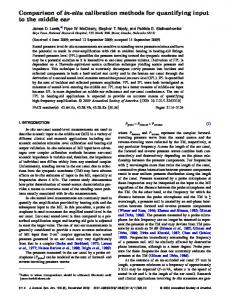
1.1 Description Currently, genuine local approach is still the most commonly used process to calibrate production engines. The emission calibration workflow for this well known approach is divided into three steps: – a preliminary phase consisting in choosing the operating points (OP) to work on and corresponding emissions targets; – the optimization of engine responses on each OP according to these targets; – the map building after smoothing between these optimal settings. The preliminary step starts with gathering the compulsory documentation regarding the vehicle (inertia, aerodynamics, etc.), the gearbox (gear ratio, internal frictions, etc., the engine (components specifications, etc.), the driving cycle and the development targets. This phase is a prerequisite for the identification of the corresponding path of the emission cycle in the speed-load area. Then assuming a certain number of hypotheses, such as neglecting the transient effects on the accelerations of the NEDC (i.e. to consider them as the sum of stabilized points), it is possible to sample the cycle and select specific points representing this cycle in the engine working range. Figure 1 gives an example of NEDC simulation and a selection of 17 OP. As the set of OP should represent the overall driving cycle, it is necessary to describe how each OP contributes as a fraction of the whole cycle. A time weight is thus affected to each OP, the sum of these weights being equal to the

10

100

8

10 Hz cycle trace Operating points

NEDC cycle 80

BMEP (bar)

Vehicle speed (km/h)

120

60

6 4

40

2

20

0

0 0

200

400

600 Time (s)

800

1000

Figure 1 Cycle simulation and selection of operating points.

1200

-2 800 1000 1200 14001600 1800 20002200 2400 26002800 Engine speed (rpm)

M Castagné et al. / Comparison of Engine Calibration Methods Based on Design of Experiments (DoE)

length of all the mass emission production phases during the cycle. The calculation of time weights is merely based on the center of gravity determination principle, in the speed-load area. The next task is the determination of allocations for all engine responses on every OP, i.e. the upper bound of each engine response in order to guarantee the cumulated level of emissions on the cycle and the desired level of combustion noise. Thus defined, allocations are local constraints which will guide the optimization process. The optimization of engine responses on each OP takes place after these steps. If the number of engine control parameters is limited (for example air/fuel ratio and spark ignition timing on a naturally aspirated spark ignition engine), this local optimization can be performed manually by searching progressively the optimal value of each engine control parameters, with the help of mono dimensional variations. With an increasing number of parameters, the optimization process requires more sophisticated methods based on the use of DoE and optimization techniques. This process can be schematically divided into five steps: – Define the domain of variation of the engine control parameters. This is an essential step of the process as it defines the validity domain of the models (referred as VD hereafter). The complexity of the models to be used for engine response depends on the size of this domain: For tiny domains weak order polynomials (second order) are usually sufficient to model accurately engine responses. – Build the test matrix. Various types of experimental designs can be used to build a test matrix: D-Optimal, space filling... The choice of the type of design as well as the number of tests to be done are directly correlated with the assumed complexity

of the model and thus with the size of the considered domain [3]. D-Optimal test designs are often used with hypercubic tiny domains. – Run this test matrix on the test bench. As the tests are predefined, the experiment can be performed in an automated way, which drastically improves the productivity of the global process. In this case, special attention must be paid to the validation of the experimental data. – Model the engine responses. Various softwares are available on the market for this purpose – Optimize the engine control parameters to meet the allocations. The problem may be formulated as a classical mathematical problem of optimization under constraints or as a multiobjective optimization (searching for compromises between antagonist objectives). For the local approach, the optimization is performed one OP after the other, with considering the allocations of each OP as the constraints. A difficulty turns out to be the fact that the optimal settings are very often at the limit of the VD, if this one is too narrow. Consequently, it is often necessary to go back to the first step of the process with the present optimal settings considered as the centre of the new VD. This operation will be repeated until the new optimal settings are no more located at the limit of the VD (Fig. 2). When the optimal settings are found, the last step consists in integrating them in the reference engine maps (if available) or building maps from these settings. For the drivability of the target vehicle and because sharp evolution of air loop parameters are not easily feasible during transient, it is necessary to provide smooth engine maps. Thus, the

Parameter 2

3rd VD 2nd VD VD: Validity domain

1st optimal setting

Initial VD

2nd optimal setting Final optimal setting

Parameter 1 Figure 2 Progressive optimization.

565

566

Oil & Gas Science and Technology – Rev. IFP, Vol. 63 (2008), No. 4

Cycle simulation

INITIAL STEP

Engine application

OP choice and ponderation Emissions targets Allocations calculation

MODELLING AND OPTIMIZATION STEP

Domain definition

Too wide domain

Design of test matrix assuming a model

Test realisation

Too narrow domain

Wrong assumption on the model shape

Modelling of engine responses

Allocations NO Models accurate enough? YES Optimization under constraints NO Allocations met? YES YES

SMOOTHING STEP

Optimum at a limit of domain?

Emission targets

Smoothing under constraints

NEW ENGINE MAPS

Flow chart of the genuine local method.

Maps shape NO

Satisfying result? YES

Figure 3

NO

567

M Castagné et al. / Comparison of Engine Calibration Methods Based on Design of Experiments (DoE)

settings are often moved away from their optimal values in order to build smooth engine maps, especially for air loop parameters. This smoothing process can be performed with respect to local constraints (such as maximum gradients), as well as to keep some predefined shapes. The difficulty of this step is thus to stay as close as possible to the local optima while keeping a smooth map shape, in order to keep all the benefits of the optimization work and satisfy the targets. The different steps of the method are synthesized in Figure 3. 1.2 Discussion This approach offers several advantages such as its simplicity, the precision of the models (especially for tiny domains) and the ability to obtain easily very satisfying local optimal settings thanks to slight modifications of the tuning of a previous engine. These are the reasons why this method is still used very often today. Nevertheless this method suffers from a main disadvantage: the final smoothing step after independent local optimizations can be very time consuming and the result disappointing. If the initial settings of parameters of the OP are far from each other, smoothing the maps around optimal settings is very difficult. On one hand, if the smoothing constraint is weak, drivability problems can be encountered during transient operations due to sharp steps between the settings used in the engine control. Moreover, the settings between the calibrated OP can be far from their optimal values (if the engine response against control parameters is not linear), which can result in surprising results when playing the NEDC. On the other hand, if the smoothing degree is high, parameters move away from the optimal settings and the cumulated emissions, fuel consumption as well as the combustion noise, cannot then satisfy the objectives any more. In such a case, the optimization and smoothing process must be carried out again with new constraints in order to bring the optimal settings of the various OP closer to each other, taking the risk that the new optima reach the VD limits. In the worst case, if no satisfying maps can be found, it can be necessary to run the whole process again from the very first step (allocations calculation). Depending on the number of iterations to find satisfying maps, it is obvious that the process can be quite long.

Smoothing step consists in integrating optimization results within original maps. The resulting maps should remain smooth, while keeping the value of the parameters as closed as possible to optimized values. To ensure this constraint, tolerances are predefined around optimal tunings. A first tool has been designed to calculate these tolerances on engine tunings from criteria on cumulated responses (for instance +4% for particulate emissions). It uses statistical models of the engine responses, as well as OP weighting. The chosen tolerance on cumulated response δSumResp is written as a weighted (weights WOPj defined in Sect. 1.1) cumulated sum of local responses associated with each OP: δSumResp = ∑ WopOPj δRespOPj    with    j ∈ {1,  2, ...,  card (OPj )} OPj

and    Resp = Resp( pi )   with    i ∈ {1,  2, ...,  card ( pi )}

Furthermore: ∀OP : δResp = ∑ i

When considering an equal mean contribution of each parameter at each OP to cumulated response and by identifying each term of these two sums δSumResp =

As the smoothing step has been identified as the most critical phase of the whole process, we developed specific tools in order to make this operation as easy as possible and prevent one from performing it blindly.

1

δSumResp =

1

∑ ∑ card (OP ) card ( p ) j

OPj i

∑ WOP ∑ j

OPj

i

∂RespOPj ∂pi

i

δpiOPj

we obtain: δpiOPj =

δSumResp ∂RespOPj × card ( pi ) * card (OPj ) WopOPj × ∂pi

Figure 4 summarizes the principle of this method. The second tool builds a smooth map of each control parameter (with or without an original map) using the optimal tunings on the (discrete) OP and predefined tolerances (obtained from first tool). The method minimizes curvature mismatch between solution map and initial map, while keeping tunings inside predefined tolerances: min

1.3 Specific Development Work: Smoothing Methodology

∂Resp × δpi at first order ∂pi

∂2 m( N , Qinj ) ∂2 m INIT ( N , Qinj ) − ∂N 2 ∂N 2

2

∂2 m( N , Qinj ) ∂2 m INIT ( N , Qinj ) − + ∂Qinj 2 ∂Qinj 2 +

∂m( N , Qinj ) ∂2 m INIT ( N , Qinj ) − ∂N ∂Qinj ∂N ∂Qinj

2

2

568

Oil & Gas Science and Technology – Rev. IFP, Vol. 63 (2008), No. 4

Original map

Optimal settings

Final map

Tolerance on tuning

Figure 4 Principle of IFP smoothing method.

Smoothed Map Tight criterion

Initial Map

x 105 Injection pressure (hPa)

Injection pressure (hPa)

x 105 15 10 5 0

15 10 5 0

80 60 40

Injected 20 quantity (mg/st)

80

5000 4000 3000 Engine 2000 speed (rpm) 0 1000

60 40

Injected 20 quantity (mg/st)

Smoothed Map Relaxed criterion

Initial Map

x 105 Injection pressure (hPa)

x 105 Injection pressure (hPa)

5000 4000 3000 Engine 2000 speed (rpm) 0 1000

15 10 5 0

15 10 5 0

80 60 40

Injected 20 quantity (mg/st)

0 1000

2000

3000

Figure 5 Examples of smoothing with different criteria.

4000

5000

Engine speed (rpm)

80 60 40

Injected 20 quantity (mg/st)

0 1000

2000

3000

4000

5000

Engine speed (rpm)

M Castagné et al. / Comparison of Engine Calibration Methods Based on Design of Experiments (DoE)

With constraint: εi1 ≤ m( N i , Qiinj ) − m INIT ( N i , Qiinj ) ≤ εi 2   ∀i with: – (Ni, Qiinj) is the coordinate of optimized OP; – εi are tolerances calculated with specific tool presented above; – m and mINIT are respectively solution and initial map. Consequently, for large tolerances, the shape of the final map will be closed to the shape of the initial map whereas the tunings at discrete optimized OP are allowed to be far from optimal tunings.

Figure 6 Screen shot of IFP map building and cumulated emission estimation tool.

569

Figure 5 presents smoothing results for injection pressure map with different tolerance definition criteria. At the top of the figure, the criterion is a 2% penalty for particle emissions. On the left the initial map is displayed, with optimal tunings for each OP superimposed in green, and tolerances are shown in pink. On the right, the solution map is closed to optimal tunings, but it is not as regular as the initial map. Below, the presented result corresponds to a criterion of 20% penalty on particle emissions. With this relaxed criterion, injection pressure can be significantly reduced, as shown with wide tolerances around optimal tunes. Then, final map is smoother than the previous one, but settings are relatively far from optimal ones.

570

Oil & Gas Science and Technology – Rev. IFP, Vol. 63 (2008), No. 4

The main idea of the third tool is the use of statistical models of the engine responses on each OP to visualize the sensitivity of the responses with respect to each parameter, and evaluate the effects of the tolerances around the optimal settings on engine responses. This tool is also used to visualize the shape of the maps after smoothing, to correct manually each map if necessary and to estimate the global level of emissions and fuel consumption over the cycle immediately after smoothing. Thus, several smoothing trials can easily be done in order to determine the most appropriate one. Figure 6 shows a screen shot of this tool. Results obtained with these tools are presented in Section 4.3 in comparison with the mixed local approach. 1.4 Conclusion for the Genuine Local Approach This approach has proved to be efficient in the industry, because the local models are accurate enough to qualify robustness, and because the results of previous engines can be used for following ones, limiting the risk during the local allocations definition and the smoothing steps. Even if improvements can be proposed, these steps remain the main drawbacks of this method, especially for tuning a new technology engine without any existing reference. Considering all these disadvantages other approaches have been investigated in order to carry out the calibration process in a more integrated way. 2 MULTI-POINTS LOCAL APPROACH 2.1 Description This method is the first level of integration and consists in optimizing several OP together in order to optimize simultaneously a more significant part of mass emissions of the cycle and avoid big variations of the resulting optimal settings on these OP. The multi-points method is equivalent to the local method until the optimization step. The optimization philosophy considers that a group of points is to be optimized, the points of the group interacting with each other. Therefore, allocations start to become global constraints or at least regional constraints. The points considered as a group will typically be concentrated in an area with a similar physical behavior of the engine or a similar tuning of several parameters (for example it is possible to assemble OP with the same engine speed or the same engine load). The number of points to be considered together for the optimization is let to the user’s judgment. The allocations calculated for this method depend on the points that will be optimized together. As one point may increase the level of emissions of one pollutant on one side and reduce the level of emissions of another pollutant on the

other side while an other point will do the opposite, this optimization offers more degrees of freedom than the local optimization: The final step of the method consists then in interpolating and/or smoothing the results inside and between the optimized OP. 2.2 Discussion This approach keeps the precision of local models and gives the advantage of a beginning of integration. The optimization is considered as a «team work» as gains on one side compensates losses on the other side. Moreover smoothing constraints are introduced in order to avoid sharp variations of engine settings from one OP to the other. However, defining these constraints may be difficult if the distance between the operating points is large. It must be mentioned that a limitation of this method (just as the previous one) lies in the size of the VD. This domain still being limited, the probability to find optimal settings on its limits is still high. The deliverables of this optimization process remain individual settings at chosen operating points: engine maps still need to be built even if this process is simplified. 2.3 Conclusion for the Multi Points Local Approach In the end this method should provide improved results thanks to the introduction of smoothing constraints but the definition of those constraints as well as the allocations (depending on the considered OP to be optimized simultaneously) is much more complex than the definition of the constraints and allocations in the genuine local method. Moreover it still faces the smoothing issue. Because of these drawbacks IFP does not consider this method as a sufficient improvement and prefers to go directly one step further in the integration process with the use of the mixed local approach. 3 MIXED LOCAL APPROACH 3.1 Description This method represents a further step in the integration process. The parameters to be optimized are not any more the parameters at chosen OP but the engine maps themselves. The optimization is then considered as a global process with an integrated smoothing. As for local approach, the emission calibration workflow could be divided into three steps, as it appears in Figure 7. Note that the preliminary phase is now limited to the choice of the OPs, performed, as previously, after a NEDC cycle simulation. Allocations are no more required because the optimization is directly made on the emission and fuel

INITIAL STEP

M Castagné et al. / Comparison of Engine Calibration Methods Based on Design of Experiments (DoE)

Engine application

571

Cycle simulation

OP choice and ponderation

MODELLING STEP

Domain definition Too wide domain

Design of test matrix assuming a model

Test realisation

Modelling of engine responses

Too narrow domain

Models accurate enough? YES

NO

Map optimization under constraints

Emission targets

SMOOTHING STEP

Wrong assumption on the model shape

Maps shape

YES Optimum at a limit of domain? NO NO Satisfying result? YES NEW ENGINE MAPS

Figure 7 Flow chart of the mixed local method.

consumption levels calculated as the sum of model responses using time weights for each OP. The optimization requires to model the engine map. Different techniques can be used for this purpose as polynomial functions, Local Linear Mode Tree (LoLiMoT), splines, etc. The smoothing constraints are applied directly on these modeled maps. Reference maps from other engines may also be used to define the expected smoothing degree of the optimized maps. 3.2 Discussion This method avoids the expensive “trial and error” smoothing step necessary in the local optimization method and removes

the need of allocations determination, which is a very difficult and risky step. Another advantage lies in the ability to use reference maps (already tested on similar engines) to define the smoothing constraints. However using local models of engine responses still leads to the same limitations as mentioned for the previous methods, namely the size of the VD of the local models and the lack of models between the various OPs. Using too narrow domain of validity of local models is risky as it potentially rises the time needed to perform the whole process. Conversely enlarging the VD of the models involves other aspects of the process, such as the number of points needed for each DOE test in order to model the engine responses at the chosen OP. Indeed, the larger the VD, the

572

Oil & Gas Science and Technology – Rev. IFP, Vol. 63 (2008), No. 4

more complex engine responses functions may be needed (for example higher degree of polynomials or any other complex functions) to preserve the precision of the models. This will be discussed in the next chapter. The lack of models between OP still brings a risk of unsuitable settings of control parameters outside these points, what is uneasy to detect before performing the final tests.

LoLiMoT models ([1, 2]) seem to be a good compromise between flexibility, accuracy and complexity: some very simple local models (linear or bilinear) are combined by a weighted sum:

3.3 Specific Development Work: Map Optimization

where the weights φi (N, Qinj), normalized Gaussian functions, control the degree of smoothness of the global surface. This representation allows an adaptive refinement of the surface: the patching associated with the definition domains of the local models may be refined during the optimization process. A finer patching allows a finer optimization (the number of degrees of freedom being increased) but may lead to a cumbersome optimization of a large number of

M

m( N , Qinj ) = ∑ (ωi0 + ωi N + ωi Qinj )φi ( N , Qinj ) i =1

For direct optimization of engine maps, an adequate set of parameters has to be chosen for these maps: this parameterization must be flexible enough to model the very different shapes of engine map surfaces (Fig. 8) and should not require too many parameters to limit the number of unknowns in the optimization process.

1

2

Main injection timing

10

Load

5 0 -5 60 4000 3000 2000 Engine 1000 speed (rpm)

40 Load

20

Engine speed Boost pressure

Load

2200 2000 1800 1600 1400 1200 1000 60 40 Engine speed

Figure 8 Examples of LoLiMoT parameterization of engine map.

Load

20 0

1000

2000

4000 3000 Engine speed (rpm)

M Castagné et al. / Comparison of Engine Calibration Methods Based on Design of Experiments (DoE)

parameters. The parameterization, namely the patch definition for LoLiMoT description of the maps should reflect the degree of smoothness the user expects for the maps: for some parameters like boost pressure, the map should remain smooth, for others like main injection timing, the smoothing constraint is not as strong. From some reference engine maps or some a priori information, a LoLiMoT parameterization of each map of engine tunings is defined (Fig. 8). The unknowns of the optimization are the LoLiMoT parameters (coefficients of local linear models ωij). The objectives to be optimized (or constrained) are the engine responses cumulated on the considered driving cycle: in this mixed approach, the cumulated responses are still the weighted sums of the local models defined at chosen representative OP. Additional smoothing constraints such as global smoothing constraints (to keep the regularity of the

original maps) or more local constraints (for example limits on the gradients of the maps) can also be introduced. Tests have been processed in order to validate this method and compare the results to the genuine local method. The DoE relies on a D-optimal design and the NEDC has been divided into 17 OP. Engine responses have been modeled using quadratic models and considering the interactions between all 5 to 6 engine control parameters (boost pressure, air mass flow rate, fuel injection pressure, pilot injection quantity, pilot and main injection timings). The emissions are measured downstream of the turbine. An optimization then been processed with the following target: the production maps being focused on the minimization of the NOx emissions to the detriment of the particulate matters (PM) emissions, we decided to minimize the PM, allowing a maximum increase of NOx emissions of 10% above the nominal level measured using the original maps of

Pilot quantity (mg/st)

Initial map

Initial map

5 4 3 2 1

0 80 60 40 Injected quantity (mg/st)

20 0 0

1000

2000

Genuine local method

Figure 9 Comparison of pilot injection quantity maps.

3000

573

4000

Engine speed (rpm)

Mixed local method

574

Oil & Gas Science and Technology – Rev. IFP, Vol. 63 (2008), No. 4

Emissions considered here are NOx emissions and PM emissions. The small dots represent the points one has been working on. The table shows the differences between the initial and optimized cumulated emissions levels on the overall NEDC with both methods. Cumulated emissions are calculated using time weights and the level of emissions measured on each operating point. As one can see, the experimental results agree with the expected ones. With the genuine local method and using computed assisted smoothing, it has been possible to improve significantly (more than 30%) the level of particulate matter emissions (PM) without worsening too much the NOx

the engine control parameters. An optimization has been performed with the genuine local method with the same objectives, using the specific smoothing tools presented previously. Figure 9 shows a comparison of pilot quantity maps resulting from the optimization and smoothing processes. The impacted area is encircled. Figure 10 presents the results obtained with the genuine local method and with mixed local method. Each graph represents the differences between the levels of emissions measured engine running on its production engine control maps and engine running on its optimal engine control maps.

Gains on emissions compared to original settings NOx

PM

HC

CO

CO2

Genuine local

10.3

-31.4

24.3

1.9

-1.0

Mixed local

5.5

-30.5

50.1

23.1

-1.9

NOx emissions Differencies between genuine local and initial maps (%)

Particulates emissions Differencies between genuine local and initial maps (%) 10

10

30

30 8

8

10

6

5

4

-5

BMEP (bar)

BMEP (bar)

10 6

5

4

-5 -10

-10 2

2

-30

-30 0 1000

1500

2000 2500 Engine speed (rpm)

0 1000

3000

NOx emissions Differencies between mixed local and initial maps (%)

1500

2000 2500 Engine speed (rpm)

3000

Particulates emissions Differencies between mixed local and initial maps (%) 10

10

30

30 8

8

10

6

5 -5

4

BMEP (bar)

BMEP (bar)

10 6

5 -5

4

-10

-10 2 0 1000

-30 1500

2000 2500 Engine speed (rpm)

3000

Figure 10 Comparison of emissions levels between initial and optimized settings.

2 0 1000

-30 1500

2000 2500 Engine speed (rpm)

3000

M Castagné et al. / Comparison of Engine Calibration Methods Based on Design of Experiments (DoE)

emissions, those being around the optimization constraint of a 10% increase. The specific consumption remains more or less at its original level but it seems that the optimal settings largely worsen the level of unburned hydrocarbons (HC) emissions. The mixed local method shows the same potential of reduction of the PM emissions (–30%) with a better result on the NOx emissions (+5.5%). However HC and CO emissions are worse than those obtained with the manual local method. These results could probably be improved by strengthening the constraints on HC and CO emissions for the combined optimization and smoothing process. It is interesting to notice that the results reflect the optimization process. The map optimization uses the global result on NEDC whereas the local method optimizes the operating points one by one before smoothing and worsening the gains, which is why gains and losses are not at the same points on the presented emissions maps. Furthermore, engine control maps obtained with both methods are smooth enough. Yet the mixed local method does have the major advantage of being much less time consuming. Time gains make it possible to try various optimization objectives and test it on the test bed to find the most suitable settings. 3.4 Conclusion for the Mixed Local Approach This approach is very attractive because it keeps the precision of local models (allowing their use to qualify robustness) and brings the advantages of integrating smoothing constraints into the optimization phase. The optimization process is then much faster and reliable. Another advantage lies in the ability to use existing maps as references for the optimization. Nevertheless this approach suffers, as the previous ones, from the limitations due to the use of local models. 4 INDIRECT GLOBAL APPROACH 4.1 Description The principle is to merge the local models with each other to build a global model, integrating load and engine speed as parameters. The optimization step can then be performed with the help of a maps global optimization technique as in the mixed local approach. Figure 11 describes the flow chart of this method. Several techniques are possible to perform the model merging: if polynomials are used for local models, a global model may be built by making the polynomial coefficients depend on engine load and speed. For a high number of coefficients (high order polynomial and/or high number of engine parameters) this method becomes cumbersome. Another way to build a global model is to sum the local models with weights depending on engine speed and load. This later approach offers more flexibility in the local model definition

575

(different types of local models may be used) and the number of weights only depends on the number of OP (and not on the number of coefficients of the local models). For both cases, the functions of load and speed may be polynomials or more complex functions. The goal of the optimization is still to minimize emissions and fuel consumption over the cycle (while preserving the combustion noise), but the evaluation of pollutant masses is here performed considering the driving cycle trace instead of a weighted sum of results on local operating points. 4.2 Discussion This method tries to avoid the drawbacks of the previous methods while keeping its advantages. The first modeling step is achieved on local domains, which makes it possible to limit the test duration and minimizes the risk of engine drift as well as a test interruption. The optimization is here performed on a model representing the whole cycle area. Fuel consumption and pollutants to be minimized are calculated on the real cycle trace instead of time weighted OP, which is much more precise and reliable (even if the assumption that emissions during transient phases are the sum of stabilized emissions on local operating points remains). If the principle of merging local models is very attractive and sounds simple, the effective achievement is much more difficult. One of the main difficulties lies in the determination of the VD of the models for each OP which must be large enough to insure a possible merging (compatibility between the OPs) and narrow enough to precisely model engine responses. IFP focused its efforts on this specific point. 4.3 Specific Development Work: Domain Definition When using hypercubic VD, the local approach supposes that no physical limit is reached in this area. Enlarging the VD for merging purpose leads to take into account physical limits in some directions and then to modify the VD shape. After testing iterative approach as Rapid Hull Determination [4], we decided to develop a simpler and more physical approach to find the limits of VD. A specific space design algorithm has been developed and implemented on the test bench in order to automatically evaluate constraints in the 2D space (air mass flow / boost pressure) according to other sets of parameters with a limited number of measuring points. Figure 12 shows what limits are reached with this algorithm in the case of a Turbo-Diesel engine with an adding intake throttle. Three of them are physical limits led by air loop permeability. The last one is much more difficult to determine since it is not physical. A way to determine it is to define some criteria about engine response or behavior. Thus, maximum level of smoke, maximum air fuel ratio

576

INITIAL STEP

Oil & Gas Science and Technology – Rev. IFP, Vol. 63 (2008), No. 4

Engine application

Cycle simulation

OP choice

Domain definition

Too wide domain

Design of test matrix assuming a model

Test realisation

Wrong assumption on the model shape

MODELLING STEP

Modelling of local engine responses

NO Local models accurate enough?

Too narrow domain

YES Building of a global domain

Building of a global model Additional tests NO

MAP OPTIMIZATION STEP

Global model accurate enough? YES Map optimization under constraints

Emission targets

YES Optima at a limit of domain? NO Satisfying result? YES

NEW ENGINE MAPS

Figure 11 Flow chart of the indirect global method.

Maps shape

NO

M Castagné et al. / Comparison of Engine Calibration Methods Based on Design of Experiments (DoE)

577

Boost pressure Maximal boost pressure

Engine response limit

Maximal air filing

Throttle closing

Minimal boost pressure Air flowrate

Figure 12 Determination of the limits of validity domain in the boost pressure / air flow rate plan.

2000

0 -2 -4 -6 -8 300

1500 400 1400 500 1300 600 1200 700 1100 Air mass Boost 800 900 1000 flow (mg/st) pressure (mbar)

Boost pressure (mbar)

Start of injection (deg. BTDC)

1900 1800 1700

1500 rpm - 5 bar 1500 rpm - 7 bar 1750 rpm - 5 bar 2000 rpm - 5 bar 2000 rpm - 7 bar

1600 1500 1400 1300 1200 1100 1000 900 150 250 350 450 550 650 750 850 950 1050 Air mass flow (mc/cyc)

Figure 13

Figure 14

Example of 3D modeling of a local domain.

Validity domain shape evolution with engine speed and BMEP.

value or also limit of stability has to be chosen, and the VD limit is obtained when one of these criteria is reached. Tests are processed to find these limits for the most critical combinations of other parameters in order to build a complete VD. After processing the experiments, we have the ability to model the constraint area for all direction. The main idea is to model the maximum and minimum limit for each variable: ymin ( p1 , … ,  pn ) ≤ y ≤ ymax ( p1 , … ,  pn ) where y is a variable and ( pi )i =1, …,  n are the other variables distinct from y.

A good model approximation for an OP is the linear model that can be expressed as followed: n

n

i =1

i =1

ymin = a0 + ∑ ai pi and ymax = b0 + ∑ bi pi The linear model coefficients (ai)i = 0, ..., n and (bi)i = 0, ..., n are estimated from experiments of the specific space design algorithm implemented on the test bench. In the case of hypercubic limits, we have ymin and ymax = b0. An example of result for an OP is illustrated in Figure 13. The further step of this methodology is to merge local VD in order to define global VD. This step is difficult since VD

578

Oil & Gas Science and Technology – Rev. IFP, Vol. 63 (2008), No. 4

shape evolutes while engine speed and break mean effective pressure (BMEP) are changing. This evolution has been studied in order to determine models type that could match global VD definition. Figure 14 shows VD evolution for several OP with different BMEP and different engine speed. The maximal air filling limit does not move significantly with engine speed and BMEP variations, since it is imposed by engine permeability. Minimal and maximal boost pressure limits seem to keep same slope for every OP and they evolve in a homogeneous way with engine speed and BMEP. The minimal air mass flow limit is varying significantly from one OP to the other, but keeps the same shape. It is noteworthy that for low BMEP OP, boost pressure amplitude for minimal air mass flow value is very low. Thus, regarding these low BMEP OP, VD is defined in the 2D space (air mass flow/ variable nozzle turbine (VNT) position demand) instead of (air mass flow/boost pressure). This way simplifies VD shape since VNT position demand limits do not change while air mass flow is varying. Non linear models have been evaluated with success in a large engine working range. ymin ( N , L, p1 , … ,  pn ) ≤ y ≤ ymax ( N , L, p1 , … ,  pn ) where N and L represent, respectively, the engine speed and load. Here, we propose a quite simple model as followed: n ⎛ ⎞ ymin = ⎜⎜ a0 + ∑ ai pi ⎟⎟ (α 0 + α1 N + α 2 L ) ⎝ ⎠ i =1

and

4.4 Conclusion for the Indirect Global Approach This approach gives the advantages of using global models in optimization, while limiting the risks during the tests by using local domains. These domains have to be defined very carefully in order to satisfy simultaneously the precision and the compatibility requested to merge the models. However, this method suffers from global test duration as well as from the complexity of the merging phase and the loss of precision of the resulting models. If the use of global models is a great improvement for the optimization process, the accuracy of local models can be used to qualify robustness around optimal settings. Note also that in addition to their advantages for optimization, global models could be used for the application of the

1800

1800

1700

1700

1600 1500 1400 1300 1200 1100 1000 900 900 1000 1100 1200 1300 1400 1500 1600 1700 1800 Estimated boost pressure (mbar)

Measured boost pressure (mbar)

Measured boost pressure (mbar)

n ⎛ ⎞ ymax = ⎜⎜b0 + ∑ bi pi ⎟⎟ (β0 + β1 N + β2 L ) ⎝ ⎠ i =1

Experimental correlation diagram shows a good prediction of the three physical limits in the 2D space (air mass flow/ boost pressure) for many OP. Figure 15 and Figure 16 give an example of these correlations for the boost pressure and the maximum air mass flow. The minimal air flow limit model is divided into two areas (low BMEP and mid BMEP OP) since boost pressure is managed differently for these two zones, in accordance with VD definition described previously. Figure 17 presents results for minimal air flow correlation: Results are reasonably good for the two zones since using VNT position demand as parameter instead of boost pressure really improved model quality. Furthermore, it is significant that criterion used to determine minimal air mass flow limit has to be defined in a homogeneous way from one OP to the other in order to get a smooth VD shape evolution and to avoid problems when merging the local models.

1600 1500 1400 1300 1200 1100 1000 900 900 1000 1100 1200 1300 1400 1500 1600 1700 1800 Estimated boost pressure (mbar)

Figure 15

Figure 16

Evaluation of the global model prediction of maximum (red) and minimum (black) boost pressure.

Evaluation of the global model prediction of maximum air mass flow.

M Castagné et al. / Comparison of Engine Calibration Methods Based on Design of Experiments (DoE)

Several kinds of models can be used for each of these regional domains, such as LoLiMoT models, which require a space filling DoE (Latin Hypercube for instance) [6]. – The optimization step, which is the same as in the previous approach. Map optimization appears clearly as the most appropriate way to define optimal settings all over the engine speed and load domain. Figure 18 shows the flow chart of this method.

550 500 Measured boost pressure

579

450 400 350 300 250

5.2 Discussion 200 200

250

300 350 450 500 400 Estimated air mass flow (mg/cyc)

550

Figure 17 Evaluation of the global model prediction of minimum air mass flow.

same engine in several vehicles. It will be sufficient to perform a new optimization on an other engine speed-load trace, and, if necessary, with other objectives regarding combustion noise and fuel consumption. 5 GENUINE GLOBAL APPROACH 5.1 Description This method suppresses the local modeling step. Models of engine responses are built directly on the overall driving cycle area, load and engine speed considered as parameters. As previously the method can be divided into three steps: – The initial step, which is now reduced to the simulation of NEDC cycle. The modeling step, which is the most difficult and time consuming step. Searching the global domain in which model will be built is a very important part of this step, which requires a great effort. The test matrix is thus much larger and the test can last very long. Special attention must consequently be paid to engine and test equipment drifts. To limit the risk during modeling, it is recommended to split the design space into several regions with homogeneous settings, for which different models can be used (for example to divide the {engine speed, load} domain according to the kind of injections or the combustion mode). Models are merged in order to build a multiple-region model. Interpolations between the models at their boundaries are then required to insure a smooth transition [5].

As in the previous approach, it is difficult to obtain a precise model on a large domain. The determination of the domain can be long and difficult. Another drawback of this method is the duration of the engine test to fulfill the multidimensional parameter space with a sufficient number of measurements, which can cause engine and test equipment drifts. As mentioned before, it is advisable to divide the domain into more local areas with homogeneous settings in order to limit these drawbacks. Another major improvement could be added for model accuracy by the use of one-line modeling [6]. Reduction of test duration can also be obtained by the use of deconvolution techniques in order to avoid the stabilization period before the measure. 5.3 Conclusion for the Genuine Global Approach Because of the size of the experimental domains the effective achievement of this method is quite difficult and risky, and requires strong precautions during tests and modeling phases. Nevertheless if the above drawbacks can be overcome, this approach is the ultimate step of integration with all the advantages brought by a global approach: information available on the whole cycle area for optimization, integrated smoothing, and a limited number of steps are necessary to produce optimized engine maps. Getting sufficiently accurate models to qualify the robustness of the optimal settings to engine, transducers and actuators variations in production is probably the main challenge of this method. 6 SYNTHESIS OF EXPERIMENTAL APPROACHES Considering each approach as a whole, it must be underlined that the test duration is only a part of the global duration of each process. The off-line analysis work can actually be very time consuming, especially in the processes with a high number of steps (local or semi local methods). This phenomenon can be amplified if the process must be fully or partially done again, due to the insufficient size of local domains or too big

580

INITIAL STEP

Oil & Gas Science and Technology – Rev. IFP, Vol. 63 (2008), No. 4

Engine application

Cycle simulation

MODELLING STEP

Domain definition

Too wide domain

Design of test matrix

Test realisation

Too narrow domain

Wrong assumption on the model shape

Modelling of engine responses

NO Global model accurate enough? YES Map optimization under constraints

SMOOTHING STEP

Emission targets

Maps shape

YES Optimum at a limit of domain? NO NO Satisfying result? YES

NEW ENGINE MAPS

Figure 18 Flow chart of the genuine global method.

losses of optimality during smoothing. When comparing the approaches, these considerations must be kept in mind. All the approaches are summarized in Table 1 with their main advantages and drawbacks. If development time does not appear directly in the previous table, integrated smoothing and reduction of steps for modeling bring clearly a gain in this very important matter. Major improvement in development time is also brought by the re-use of existing model when engine must be optimized for an other vehicle application. Two kinds of questions rise from discussions about the accuracy of the models: do the models give the good

tendencies on engine responses with respect to control parameters? Are engine responses predicted with a great accuracy? A positive answer to the first question allows to use the models for a first level of optimization. A positive answer to the second question allows to use them to finalize the optimization and to qualify the robustness of optimal settings to variations in production. An appropriate development scheme can consist in building a first level of engine model to perform a first optimization and then refining progressively this model in order to finalize this optimization and qualify its robustness. This progressive approach of model based development can

581

M Castagné et al. / Comparison of Engine Calibration Methods Based on Design of Experiments (DoE)

TABLE 1 Synthesis of the experimental approaches Approach

Genuine local

Multi point

Mixed

Globalindirect

Genuine global

Kind of model of engine responses

Local models

Local models

Local models

Merging of local models

Global models

Optimization and maps building

Local optimization + smoothing

Multi-points optimization + inerpolation

Global optimization of maps

Global optimization of maps

Global optimization of maps

Main advantages

Precision of local models

Precision of local models

Precision of local models

Model available for every applications of the engine

Model available for every applications of the engine

Simplicity

Some smoothing constraints

Integrated smoothing Information on the whole cycle area

Information on the whole cycle area

Integrated smoothing

Integrated smoothing

Two levels of models

Few steps

Main drawbacks

No information between OP

No information between OP

No information between OP

Imprecision of global models

Imprecision of global models

Lots of steps

Lots of steps

Numerous steps

Numerous steps

Risk of drift during test

Loss of optimality during smoothing

Small loss of optimality during smoothing

consist in using a global approach in a first step. The second step can consist in performing additional tests around optimal settings in order to build accurate local models or refine the global models. Use of physical engine simulation can be another efficient way to perform the first step. 7 USE OF PHYSICAL MODELS IN CALIBRATION Increasing the use of physical models together with statistical models seems to be a very clear tendency for model-based calibration [7]. IFP is developing, with its partner Imagine, a full chain of engine and vehicle simulation tools in the platform AMESim‚ which can enter in the calibration process. Regarding the tuning of control parameters in stabilized conditions, for which the calculation time is not a key parameter, it is possible to use variable step time solvers, allowing the use of sophisticated physical models. Genuine physical models can also be used for an engine pre-calibration. This pre-calibration can occur in a very advanced phase of development, as soon as some prototype engine tests are available to qualify the models. As the experimental calibration process is moving forwards, it is progressively possible to combine statistical models and physical ones or to use the results of statistical models to adjust physical ones in order to obtain a better match between modeling and experimental results.

Complexity

But the key challenge regarding the use of physical models (combined with statistical ones) is probably in the field of transient calibration. Indeed the actual responses of air loop parameters during transient can be far from their responses during stabilized conditions. For example turbo lag induces a delay in the rise of boost pressure and in the decrease of exhaust gas recirculation (EGR) rate during vehicle acceleration. The hypothesis of stabilized conditions used to calibrate the parameters during the acceleration phases of NEDC is actually far from reality. Taking into account the actual trajectory in terms of boost pressure and EGR rate during these acceleration phases brings a big improvement in calibration results. Using physical models of air loop combined with statistical models of engine responses obtained by DoE tests could be a good way to perform a first calibration of control parameters during transient operations. CONCLUSION Facing the reduction of development schedule, the increasing complexity of engines control strategies and more stringent emissions, durability and quality requirements, the calibration phase becomes a critical step of the vehicle development process. Purely «trial and error» approaches are no more possible to tune all the calibration parameters. The necessity of model-based development is now obvious, in order to

582

Oil & Gas Science and Technology – Rev. IFP, Vol. 63 (2008), No. 4

perform an extensive part of the development work with the use of engine and vehicle models and mathematically assisted optimization of the calibration parameters. Nowadays, engine control strategies are still essentially map based, and this paper focused on the methods used to fulfill these maps with optimal and smooth settings in the NEDC zone. Several methodologies may be followed for that purpose, from the use of the traditional genuine local approach, characterized by a phase of smoothing between local optimal settings, to the use of genuine global approaches directly including engine speed and load as parameters in models. Intermediate approaches have also to be considered. The mixed approach, combining the use of local modeling and direct map optimization techniques, and the indirect global approach in which local models are merged to build a global model seem to be the most interesting intermediate approaches. Design of Experiments and automated tests are used for each of these calibration methods. Specific developments have been performed at IFP to answer the key challenges identified to better use these methods. Each of these approaches has got advantages and drawbacks discussed in this paper and synthesized in Section 7, regarding the development time and the robustness of the optimal settings. In the end, a development scheme can be proposed, using physical simulations and/or a global approach for a first level of models and optimization, and progressive improvements of the models accuracy in order to refine the optimal settings and to be able to qualify their robustness in a reliable way.

ACKNOWLEDGEMENTS The authors would like to acknowledge Sébastien Gindre, Jean Marie Hascoet and Roland Dauphin for their contribution to this work. REFERENCES 1 Nelles O. (2001) Non linear system identification, SpringerVerlag. 2 Hafner M., Isermann R. (2001) The use of stationary and dynamic emission models for an improved engine performance in legal test cycles, International workshop on Modeling, Emissions and Control in automotive engines, Salerno, Italy. 3 Montgomery D.C., Myers R.H. (1995) Response surface methodologies: process and product optimization using designed experiments, Wiley Interscience, Wiley series in probability and statistics. 4 Renninger P., Aleksandrov M. (2005) A new method to determine the design space for model based approaches, DoE in engine development II, Berlin, Germany. 5 Röpke K., Gaitzsch R., Haukap C., Knaak M., Knobel C., Neßler A., Schaum A., Schoop U., Tahl S. (2005) DoE – Design of Experiments, Methods and applications in engine development, Verlag Moderne Industrie. 6 Buzy A., Albertelli M., Cotte P., Grall S., Visconti J. (2005) On line adaptative DOEs and global modeling for Diesel engines and DPF calibration, DoE in engine development II, Berlin, Germany. 7 Ohata A., Ehara M., Watanabe S., Butts K. (2006) Model-based design and future calibration processes at Toyota, Workshop on open problems and challenges in automotive control. Final manuscript received in November 2007 Published online in July 2008

Copyright © 2008 Institut français du pétrole Permission to make digital or hard copies of part or all of this work for personal or classroom use is granted without fee provided that copies are not made or distributed for profit or commercial advantage and that copies bear this notice and the full citation on the first page. Copyrights for components of this work owned by others than IFP must be honored. Abstracting with credit is permitted. To copy otherwise, to republish, to post on servers, or to redistribute to lists, requires prior specific permission and/or a fee: Request permission from Documentation, Institut français du pétrole, fax. +33 1 47 52 70 78, or [email protected].