Comparison of Failure Detectors and Group Membership - CiteSeerX

Comparison of Failure Detectors and Group Membership: Performance Study of Two Atomic Broadcast Algorithms (extended version) Péter Urbán†

Ilya Shnayderman‡

André Schiper†

[email protected]

[email protected]

[email protected]

´ Ecole Polytechnique Fédérale de Lausanne (EPFL), CH-1015 Lausanne, Switzerland ‡ School of Engineering and Computer Science, The Hebrew University of Jerusalem, Israel †

Technical Report IC/2003/15 Faculté d’Informatique et Communications (I&C) École Polytechnique Fédérale de Lausanne (EPFL) Abstract Protocols that solve agreement problems are essential building blocks for fault tolerant distributed systems. While many protocols have been published, little has been done to analyze their performance, especially the performance of their fault tolerance mechanisms. In this paper, we present a performance evaluation methodology that can be generalized to analyze many kinds of fault-tolerant algorithms. We use the methodology to compare two atomic broadcast algorithms with different fault tolerance mechanisms: unreliable failure detectors and group membership. We evaluated the steady state latency in (1) runs with neither crashes nor suspicions, (2) runs with crashes and (3) runs with no crashes in which correct processes are wrongly suspected to have crashed, as well as (4) the transient latency after a crash. We found that the two algorithms have the same performance in Scenario 1, and that the group membership based algorithm has an advantage in terms of performance and resiliency in Scenario 2, whereas the failure detector based algorithm offers better performance in the other scenarios. We discuss the implications of our results to the design of fault tolerant distributed systems.

1

Introduction

Agreement problems — such as consensus, atomic broadcast or atomic commitment — are essential building blocks for fault tolerant distributed applications, including transactional and time critical applications. These agreement problems have been extensively studied in various system models, and many protocols solving these problems have been published [1, 2], offering different levels of guarantees. However, these protocols have mostly been analyzed from the point of view

of their safety and liveness properties, and very little has been done to analyze their performance. Also, most papers focus on analyzing failure free runs, thus neglecting the performance aspects of failure handling. In our view, the limited understanding of performance aspects, in both failure free scenarios and scenarios with failure handling, is an obstacle for adopting such protocols in practice. Unreliable failure detectors vs. group membership. In this paper, we compare two (uniform) atomic broadcast algorithms, the one based on unreliable failure detectors and the other on a group membership service. Both services provide processes with estimates about the set of crashed processes in the system.1 The main difference is that failure detectors provide inconsistent information about failures, whereas a group membership service provides consistent information. While several atomic broadcast algorithms based on unreliable failure detectors have been described in the literature, to the best of our knowledge, all existing group communication systems provide an atomic broadcast algorithm based on group membership (see [3] for a survey). So indirectly our study compares two classes of techniques, one widely used in implementations (based on group membership), and the other (based on failure detectors) not (yet) adopted in practice. The two algorithms. The algorithm that uses unreliable failure detectors is the Chandra-Toueg atomic broadcast algorithm [4], which can tolerate f < n/2 crash failures, and requires the failure detector ♦S. As for an algorithm using group membership, we chose an algorithm that implements total order with a mechanism close to the failure detector based algorithm, i.e., a sequencer based algorithm (which also tolerates f < n/2 crash failures). Both algorithms were optimized (1) for failure and suspicion free runs (rather than runs with failures and suspicions), (2) to minimize latency under low load (rather than minimize the number of messages), and (3) to tolerate high load (rather than minimize latency at moderate load). We chose these algorithms because they are well-known and easily comparable: they offer the same guarantees in the same model. Moreover, they behave similarly if neither failures nor failure suspicions occur (in fact, they generate the same exchange of messages given the same arrival pattern). This allows us to focus our study on the differences in handling failures and suspicions. Methodology for performance studies. The two algorithms are evaluated using simulation. We model message exchange by taking into account contention on the network and the hosts [5]. We model failure detectors (including the ones underlying group membership) in an abstract way, using the quality of service (QoS) metrics proposed by Chen et al. [6]. Our performance metric for atomic broadcast is called latency, defined as the time that elapses between the sending of a message m and the earliest delivery of m. We study the atomic broadcast algorithms in several benchmark scenarios, including scenarios with failures and suspicions: we evaluate the steady state latency in (1) runs with neither crashes nor suspicions, 1 Beside masking failures, a group membership service has other uses. This issue is discussed in Section 8.

2

(2) runs with crashes and (3) runs with no crashes in which correct processes are wrongly suspected to have crashed, as well as (4) the transient latency after a crash. We believe that our methodology can be generalized to analyze other faulttolerant algorithms. In fact, beside the results of the comparison, the contribution of this paper is the proposed methodology. The results. The paper shows that the two algorithms have the same performance in run with neither crashes nor suspicions, and that the group membership based algorithm has an advantage in terms of performance and resiliency a long time after crashes occur. In the other scenarios, involving wrong suspicions of correct processes and the transient behavior after crashes, the failure detector based algorithm offers better performance. We discuss the implications of our results to the design of fault tolerant distributed systems. The rest of the paper is structured as follows. Section 2 presents related work. Section 3 describes the system model and atomic broadcast. We introduce the algorithms and their expected performance in Section 4. Section 5 summarizes the context of our performance study, followed by our simulation model for the network and the failure detectors in Section 6. Our results are presented in Section 7, and the paper concludes with a discussion in Section 8.

2 Related work Most of the time, atomic broadcast algorithms are evaluated using simple metrics like time complexity (number of communication steps) and message complexity (number of messages). This gives, however, little information on the real performance of those algorithms. A few papers provide a more detailed performance analysis of atomic broadcast algorithms: [7] and [8] analyze four different algorithms using discrete event simulation; [5] uses a contention-aware metric to compare analytically the performance of four algorithms; [9, 10] analyze atomic broadcast protocols for wireless networks, deriving assumption coverage and other performance related metrics. However, all these papers analyze the algorithms only in failure free runs. This only gives a partial understanding of their quantitative behavior. Other papers analyze agreement protocols, taking into account various failure scenarios: [11] presents an approach for probabilistically verifying a synchronous round-based consensus protocol; [12] analyzes a Byzantine atomic broadcast protocol; [13] evaluates the performability of a group-oriented multicast protocol; [14] compares the impact of different implementations of failure detectors on a consensus algorithm (simulation study); [15] analyzes the latency of the Chandra-Toueg consensus algorithm. Note that [15], just as this paper, models failure detectors using the quality of service (QoS) metrics of Chen et al. [6].

3 Definitions 3.1

System model

We consider a widely accepted system model. It consists of processes that communicate only by exchanging messages. The system is asynchronous, i.e., we make 3

no assumptions on its timing behavior: there are no bounds on the message transmission delays and the relative processing speeds of processes. The network is quasi-reliable: it does not lose, alter nor duplicate messages (messages whose sender or recipient crashes might be lost). In practice, this is easily achieved by retransmitting lost messages. We consider that processes only fail by crashing. Crashed processes do not send any further messages. Process crashes are rare, processes fail independently, and process recovery is slow: both the time between crashes and time to repair are much greater than the latency of atomic broadcast. The atomic broadcast algorithms in this paper (and all the fault-tolerant algorithms in the literature) use some form of crash detection. We call the parts of the algorithms that implement crash detection failure detectors. The failure detector based atomic broadcast algorithm uses failure detectors directly; the group membership based atomic broadcast algorithm uses them indirectly, through the group membership service. A failure detector maintains a list of processes it suspects to have crashed. It might make mistakes: it might suspect correct processes and it might not suspect crashed processes immediately.2 Note that whereas we assume that process crashes are rare, (wrong) failure suspicions may occur frequently, depending on the tuning of the failure detectors.

3.2

Atomic broadcast

Atomic Broadcast is defined in terms of two primitives called A-broadcast(m) and A-deliver(m), where m is some message. Informally speaking, atomic broadcast guarantees that (1) if a message is A-broadcast by a correct process, then all correct processes eventually A-deliver it, and (2) correct processes A-deliver messages in the same order (see [18, 4] for more formal definitions). Uniform atomic broadcast ensures these guarantees even for faulty processes. In this paper, we focus on uniform atomic broadcast.

4 Algorithms This section introduces the two atomic broadcast algorithms and the group membership algorithm. Then we discuss the expected performance of the two atomic broadcast algorithms.

4.1

Chandra-Toueg uniform atomic broadcast algorithm

The Chandra-Toueg uniform atomic broadcast algorithm uses failure detectors directly [4]. We shall refer to it as the FD atomic broadcast algorithm, or simply as the FD algorithm. A process executes A-broadcast by sending a message to all processes.3 When a process receives such a message, it buffers it until the delivery 2

To make sure that the atomic broadcast algorithms terminate, we need some assumptions on the behavior of the failure detectors [16]. These assumptions are rather weak: they can usually be fulfilled in real systems by tuning implementation parameters of the failure detectors [17]. 3 This message is sent using reliable broadcast. We use an efficient algorithm inspired by [19]. The algorithm works as follows. Consider a reliable broadcast message m sent from s to d1 , . . . , dk . s simply sends m to all destinations d1 , . . . , dk . Processes buffer all received messages for later retransmission. di retransmits m when its failure detector suspects the sender s and all destinations with smaller indexes d1 , . . . , di−1 . This algorithm requires one broadcast message if the sender is not

4

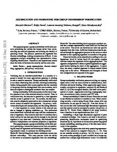
order is decided. The delivery order is decided by a sequence of consensus numbered 1, 2, . . .. The initial value and the decision of each consensus is a set of message identifiers. Let msg(k) be the set of message IDs decided by consensus #k. The messages denoted by msg(k) are A-delivered before the messages denoted by msg(k + 1), and the messages denoted by msg(k) are A-delivered according to a deterministic function, e.g., according to the order of their IDs. Chandra-Toueg ♦S consensus algorithm. For solving consensus, we use the Chandra-Toueg ♦S algorithm [4].4 The algorithm can tolerate f < n/2 crash failures. It is based on the rotating coordinator paradigm: each process executes a sequence of asynchronous rounds (i.e., not all processes necessarily execute the same round at a given time t), and in each round a process takes the role of coordinator (pi is coordinator for rounds kn + i). The role of the coordinator is to impose a decision value on all processes. If it succeeds, the consensus algorithm terminates. It may fail if some processes suspect the coordinator to have crashed (whether the coordinator really crashed or not). In this case, a new round is started. We skip the details of the execution, since they are not necessary for understanding the paper. Example run of the FD algorithm. Figure 1 illustrates an execution of the FD atomic broadcast algorithm in which one single message m is A-broadcast and neither crashes nor suspicions occur. At first, m is sent to all processes. Upon receipt, the consensus algorithm starts. The coordinator sends its proposal to all other processes. Each process acknowledges this message. Upon receiving acks from a majority of processes (including itself), the coordinator decides its own proposal and sends the decision (using reliable broadcast) to all other processes. The other processes decide upon receiving the decision message.

4.2

Fixed sequencer uniform atomic broadcast algorithm

The second uniform atomic broadcast algorithm is based on a fixed sequencer [20]. It uses a group membership service for reconfiguration in case of a crash. We shall refer to it as the GM atomic broadcast algorithm, or simply as the GM algorithm. We describe here the uniform version of the algorithm. In the GM algorithm, one of the processes takes the role of sequencer. When a process A-broadcasts a message m, it first broadcasts it to all. Upon reception, the sequencer (1) assigns a sequence number to m, and (2) broadcasts the sequence suspected (the most frequent case) and at most two broadcast messages if crashes occur but correct processes are not suspected. As for garbage collection: all processes piggyback which messages they received on outgoing messages. A message m is removed from the buffer (1) upon retransmission and (2) when its stability is detected from the piggybacked information on incoming messages. 4 Actually, we included some easy optimizations in the algorithm (reading [4] is necessary for understanding the following explanation): (1) Phase 1 of Round 1 is skipped, and (2) the coordinator sends an abort message in Phase 4 in rounds that fail, and the other processes wait for the abort message before starting a new round. The latter optimization makes sure that processes do not start Round 2 unless suspicions occur, and thus do not load the system with unnecessary messages. The result is improved performance if no suspicions occur — which is the most common case in most systems.

5

FD alg. p1

consensus coordinator / sequencer

A-broadcast(m)

proposal

t A-deliver(m)

ack

m

decision

p2 p3 p4 p5

seqnum

ack

deliver

m

non-uniform GM alg.

uniform GM alg.

Figure 1. Example run of the atomic broadcast algorithms. Labels on the top/bottom refer to the FD/GM algorithm, respectively.

number to all. When non-sequencer processes have received m and its sequence number, they send an acknowledgment to the sequencer.5 The sequencer waits for acks from a majority of processes, then delivers m and sends a message indicating that m can be A-delivered. The other processes A-deliver m when they receive this message. The execution is shown in Fig. 1. Note that the messages denoted seqnum, ack and deliver can carry several sequence numbers. This is essential for achieving good performance under high load. Note that the FD algorithm has a similar “aggregation” mechanism: one execution of the consensus algorithm can decide on the delivery order of several messages. When the sequencer crashes, processes need to agree on the new sequencer. This is why we need a group membership service: it provides a consistent view of the group to all its members, i.e., a list of the processes which have not crashed (informally speaking). The sequencer is the first process in the current view. The group membership algorithm described below can tolerate f < n/2 crash failures (more in some runs) and requires the failure detector ♦S.

4.3

Group membership algorithm

A group membership service [3] maintains the view of a group, i.e., the list of correct processes of the group. The current view6 might change because processes in the group might crash or exclude themselves, and processes outside the group might join. The group membership service guarantees that processes see the same sequence of views (except for processes which are excluded from the group; they miss all views after their exclusion until they join again). In addition to maintaining the view, our group membership service ensures View Synchrony and Same View Delivery: correct and not suspected processes deliver the same set of messages in each view, and all deliveries of a message m take place in the same view. 5

Figure 1 shows that the acknowledgments and subsequent messages are not needed in the nonuniform version of the algorithm. We come back to this issue later in the paper. 6 There is only one current view, since we consider a non-partitionable or primary partition group membership service.

6

Our group membership algorithm [21] uses failure detectors to start view changes, and relies on consensus to agree on the next view. This is done as follows. A process that suspects another process starts a view change by sending a “view change” message to all members of the current view. As soon as a process learns about a view change, it sends its unstable messages7 to all others (all the other messages are stable, i.e., have been delivered on all processes already). When a process has received the unstable messages from all processes it does not suspect, say P , it computes the union U of the unstable messages received, and starts consensus with the pair (P, U ) as its initial value. Let (P 0 , U 0 ) be the decision of the consensus. Once a process decides, it delivers all messages from U 0 not yet delivered, and installs P 0 as the next view. The protocol for joins and explicit leaves is very similar. State transfer. When a process joins a group, its state needs to be synchronized with the other members of the group. What “state” and “synchronizing” exactly mean is application dependent. We only need to define these terms in a limited context: in our study, the only processes that ever join are correct processes which have been wrongly excluded from the group. Consequently, the state of such a process p is mostly up-to-date. For this reason, it is feasible to update the state of p the following way: when p rejoins, it asks some process for the messages it has missed since it was excluded. Process p delivers these messages, and then starts to participate in the view it has joined. Note that this only works because our atomic broadcast algorithm is uniform: with non-uniform atomic broadcast, the excluded process might have delivered messages never seen by the others, thus having an inconsistent state. In this case, state transfer would be more complicated.

4.4

Expected performance

We now discuss, from a qualitative point of view, the expected relative performance of the two atomic broadcast algorithms (FD algorithm and GM algorithm). Figure 1 shows executions with neither crashes nor suspicions. In terms of the pattern of message exchanges, the two algorithms are identical: only the content of messages differ. Therefore we expect the same performance from the two algorithms in failure free and suspicion-free runs. Let us now investigate how the algorithms slow down when a process crashes. There are two major differences. The first is that the GM algorithm reacts to the crash of every process, while the FD algorithm reacts only to the crash of p1 , the first coordinator. The other difference is that the GM algorithm takes a longer time to re-start delivering atomic broadcast messages after a crash. This is true even if we compare the GM algorithm to the worst case for the FD algorithm, i.e., when the first coordinator p1 fails. The FD algorithm needs to execute Round 2 of the consensus algorithm. This additional cost is comparable to the cost of an execution with no crashes (3 communication steps, 1 multicast and about 2n unicast messages). On the other hand, the GM algorithm initiates an expensive view change (5 communication steps, about n multicast and n unicast messages). Hence we expect that if the failure detectors detect the crash in the same time by the two algorithms, the FD algorithm performs better. 7

Message m is stable for process p when p knows that m has been received by all other processes in the current view.

7

Consider now the case when a correct process is wrongly suspected. The algorithms react to a wrong suspicion the same way as they react to a real crash. Therefore we expect that if the failure detectors generate wrong suspicions at the same rate, the FD algorithm will suffer less performance penalty.

5 5.1

Context of our performance study Performance measures

Our main performance measure is the latency of atomic broadcast. Latency L is defined for a single atomic broadcast as follows. Let A-broadcast(m) occur at time t0 , and A-deliver(m) on pi at time ti , for each i = 1, . . . , n. Then latency is defined def as the time elapsed until the first A-delivery of m, i.e., L = (mini=1,...,n ti )−t0 . In our study, we compute the mean for L over a lot of messages and several executions. This performance metric makes sense in practice. Consider a service replicated for fault tolerance using active replication [22]. Clients of this service send their requests to the server replicas using Atomic Broadcast. Once a request is delivered, the server replica processes the client request, and sends back a reply. The client waits for the first reply, and discards the other ones (identical to the first one). If we assume that the time to service a request is the same on all replicas, and the time to send the response from a server to the client is the same for all servers, then the first response received by the client is the response sent by the server to which the request was delivered first. Thus there is a direct link between the response time of the replicated server and the latency L. Latency is always measured under a certain workload. We chose simple workloads: (1) all destination processes send atomic broadcast messages at the same constant rate, and (2) the A-broadcast events come from a Poisson stochastic process. We call the overall rate of atomic broadcast messages throughput, denoted by T . In general, we determine how the latency L depends on the throughput T .

5.2

Scenarios

We evaluate the latency of the atomic broadcast algorithms in various scenarios. We now describe each of the scenarios in detail, mentioning which parameters influence latency in the scenario. Parameters that influence latency in all scenarios are the algorithm (A), the number of processes (n) and the throughput (T ). Steady state of the system. We measure latency after it stabilizes (a sufficiently long time after the start of the system or after any crashes). We distinguish three scenarios, based on whether crashes and wrong suspicions (failure detectors suspecting correct processes) occur: • normal-steady: Neither crashes nor wrong suspicions in the experiment. • crash-steady: One or several crashes occur before the experiment. Beside A, T and n, an additional parameter is the set of crashed processes. As we assume that the crashes happened a long time ago, all failure detectors in the system permanently suspect all crashed processes at this point. No wrong suspicions occur. 8

• suspicion-steady: No crashes, but failure detectors generate wrong suspicions, which cause the algorithms to take extra steps and thus increase latency. Beside A, T and n, additional parameters include how often wrong suspicions occur and how long they last. These parameters are discussed in detail in Section 6.2. It would be meaningful to combine the crash-steady and suspicion-steady scenarios, to have both crashes and wrong suspicions. We omitted this case, for we wanted to observe the effects of crashes and wrong suspicions independently. Transient state after a crash. In this scenario we force a crash after the system reached a steady state. After the crash, we can expect a halt or a significant slowdown of the system for a short period. In this scenario, we define latency such that it reflects the latency of executions that are affected by the crash and thus happen around the moment of the crash. Also, we must take into account that not all crashes affect the system the same way; our choice is to consider the worst case (the crash that slows down the system most). Our definition is the following: • crash-transient: Consider that a process p crashes at time t (neither crashes nor wrong suspicions occur, except for this crash). We have process q (p 6= q) execute A-broadcast(m) at t. Let L(p, q) be the mean latency of m, averaged def

over a lot of executions. Then Lcrash = maxp,q∈P L(p, q), i.e., we consider the crash that affects the latency most. In this scenario, we have one additional parameter, describing how fast failure detectors detect the crash (discussed in Section 6.2). We could combine this scenario with the crash-steady and suspicion-steady scenarios, to include other crashes and/or wrong suspicions. We omitted these cases, for we wanted to observe the effects of (i) the recent crash, (ii) old crashes and (iii) wrong suspicions independently. Another reason is that we expect the effect of wrong suspicions on latency to be secondary with respect to the effect of the recent crash: wrong suspicions usually happen on a larger timescale.

6

Simulation models

Our approach to performance evaluation is simulation, which allowed for more general results as would have been feasible to obtain with measurements in a real system (we can use a parameter in our network model to simulate a variety of different environments). We used the Neko prototyping and simulation framework [23] to conduct our experiments.

6.1

Modeling the execution environment

We now describe how we modeled the transmission of messages. We use the model of [5], inspired from simple models of Ethernet networks [24]. The key point in the model is that it accounts for resource contention. This point is important as resource contention is often a limiting factor for the performance of distributed algorithms. Both a host and the network itself can be a bottleneck. These two kinds of resources appear in the model (see Fig. 2): the network resource (shared among 9

all processes) represents the transmission medium, and the CPU resources (one per process) represent the processing performed by the network controllers and the layers of the networking stack, during the emission and the reception of a message (the cost of running the algorithm is neglectable). A message m transmitted for process pi to process pj uses the resources (i) CPUi , (ii) network, and (iii) CPUj , in this order. Message m is put in a waiting queue before each stage if the corresponding resource is busy. The time spent on the network resource is our time unit. The time spent on each CPU resource is λ time units; the underlying assumption is that sending and receiving a message has a roughly equal cost. The λ parameter (0 ≤ λ) shows the relative speed of processing a message on a host compared to transmitting it over the network. Different values model different networking environments. We conducted experiments with a variety of settings for λ.

send receive 7

Process p j

1

CPU i (λ time units)

m

2 3

6

CPU j (λ time units)

5

receiving host

sending host

Process p i

4

Network

(1 time unit)

Figure 2. Transmission of a message in our network model.

Crashes are modelled as follows. If a process pi crashes at time t, no messages can pass between pi and CPUi after t; however, the messages on CPUi and the attached queues are still sent, even after time t. In real systems, this corresponds to a (software) crash of the application process (operating system process), rather than a (hardware) crash of the host or a kernel panic. We chose to model software crashes because they are more frequent in most systems [25].

6.2

Modelling failure detectors

One approach to modeling a failure detector is to use a specific failure detection algorithm and model all its messages. However, this approach would restrict the generality of our study: another choice for the algorithm would likely give different results. Also, it is not justified to model the failure detector in so much detail, as other components of the system, like the execution environment, are modelled in much less detail. We built a more abstract model instead, using the notion of quality of service (QoS) of failure detectors introduced in [6]. The authors consider the failure detector at a process q that monitors another process p, and identify the following three primary QoS metrics (see Fig. 3): Detection time TD : The time that elapses from p’s crash to the time when q starts suspecting p permanently.

10

p

up trust

FD at q

t

trust suspect

suspect

mistake duration TM

t

mistake recurrence time TMR Figure 3. Quality of service metrics for failure detectors. Process q monitors process p.

Mistake recurrence time TMR : The time between two consecutive mistakes (q wrongly suspecting p), given that p did not crash. Mistake duration TM : The time it takes a failure detector component to correct a mistake, i.e., to trust p again (given that p did not crash). Not all of these metrics are equally important in each of our scenarios (see Section 5.2). In Scenario normal-steady, the metrics are not relevant. The same holds in Scenario crash-steady, because we observe the system a sufficiently long time after all crashes, long enough to have all failure detectors to suspect the crashed processes permanently. In Scenario suspicion-steady no crash occurs, hence the latency of atomic broadcast only depends on TMR and TM . In Scenario crashtransient no wrong suspicions occur, hence TD is the relevant metric. In [6], the QoS metrics are random variables, defined on a pair of processes. In our system, where n processes monitor each other, we have thus n(n − 1) failure detectors in the sense of [6], each characterised with three random variables. In order to have an executable model for the failure detectors, we have to define (1) how these random variables depend on each other, and (2) how the distribution of each random variable can be characterized. To keep our model simple, we assume that all failure detector modules are independent and the tuples of their random variables are identically distributed. Moreover, note that we do not need to model how TMR and TM depend on TD , as the two former are only relevant in Scenario suspicion-steady, whereas TD is only relevant in Scenario crash-transient. In our experiments, we considered various settings for TD , and various settings for combinations of TMR and TM . As for the distributions of the metrics, we took the simplest possible choices: TD is a constant, and both TMR and TM are exponentially distributed with (different) constant parameters. Note that these modelling choices are not realistic: suspicions from different failure detectors are probably correlated. Our study only represents a starting point, as we are not aware of any previous work we could build on (apart from [6] that makes similar assumptions). We will refine our models as we gain more experience.

7 Results We now present the results for all four scenarios. We obtained results for a variety of representative settings for λ: 0.1, 1 and 10. The settings λ = 0.1 and 10 correspond to systems where communication generates contention mostly on the network and the hosts, respectively, while 1 is an intermediate setting. For 11

example, in current LANs, the time spent on the CPU is much higher than the time spent on the wire, and thus λ = 10 is probably the setting closest to reality. Most graphs show latency vs. throughput. For easier understanding, we set the time unit of the network simulation model to 1 ms. The 95% confidence interval is shown for each point of the graph. The two algorithms were executed with 3 and 7 processes, to tolerate 1 and 3 crashes, respectively. Normal-steady scenario (Fig. 4). In this scenario, the two algorithms have the same performance. Each curve thus shows the latency of both algorithms. lambda = 0.1

lambda = 1

70

70 n=3 n=7

60

50

min latency [ms]

min latency [ms]

60

n=3 n=7

40 30 20 10

50 40 30 20 10

0

0 0

100

200

300 400 500 throughput [1/s]

600

700

800

0

100

200

300 400 500 throughput [1/s]

600

700

800

lambda = 10 800 n=3 n=7

min latency [ms]

700 600 500 400 300 200 100 0 0

10

20

30 40 50 throughput [1/s]

60

70

80

Figure 4. Latency vs. throughput in the normal-steady scenario.

Crash-steady scenario (Fig. 5). With both algorithms, the latency decreases as more processes crash. This is due to the fact that the crashed processes do not load the network with messages. The GM algorithm has an additional feature that improves performance: the sequencer waits for fewer acknowledgements, as the group size decreases with the crashes. By comparison, the coordinator in the FD algorithm always waits for the same number of acknowledgments. This explains why the GM algorithm shows slightly better performance with the same number of crashes. With the GM algorithm, it does not matter which process(es) crash. With the FD algorithm, the crash of the coordinator of Round 1 gives worse performance than the crash of another process. However, the performance penalty when the coordinator crashes is easily avoided: (1) each process tags its consensus proposal with its own identifier, and (2) upon decision, each process re-numbers all processes such that the process with the identifier in the decision becomes the coordinator of Round 1 in subsequent consensus executions. This way, crashed processes will stop being coordinators eventually, hence the steady-state latency is the same regardless 12

of which process(es) we forced to crash. Moreover, the optimization incurs no cost. Hence Fig. 5 shows the latency in runs in which non-coordinator processes crash. Note also that the GM algorithm has higher resiliency on the long term if crashes occur, as the group size decreases with the crashes. E.g., with n = 7 and 3 crashes, the GM algorithm can still tolerate one crash after excluding the crashed processes, whereas the FD algorithm can tolerate none. n = 3, lambda = 0.1

n = 7, lambda = 0.1

45

80 FD and GM, no crash FD, 1 crash GM, 1 crash

40

FD and GM, no crash FD, 1 crash GM, 1 crash FD, 2 crashes GM, 2 crashes FD, 3 crashes GM, 3 crashes

70 min latency [ms]

min latency [ms]

35 30 25 20 15

60 50 40 30

10

20

5

10

0

0 0

100

200

300 400 500 throughput [1/s]

600

700

800

0

100

200

n = 3, lambda = 1

700

800

600

700

800


45


80 70 min latency [ms]

40 min latency [ms]

600

n = 7, lambda = 1

50

35 30 25 20 15

60 50 40 30

10

20

5

10

0

0 0

100

200

300 400 500 throughput [1/s]

600

700

800

0

100

200

n = 3, lambda = 10

300 400 500 throughput [1/s] n = 7, lambda = 10

700


600


800 700

500

min latency [ms]

min latency [ms]

300 400 500 throughput [1/s]

400 300 200

600 500 400 300 200

100

100

0

0 0

10

20

30

40

50

60

70

80

0

throughput [1/s]

10

20

30

40

50

60

70

80

throughput [1/s]

Figure 5. Latency vs. throughput in the crash-steady scenario. In each graph, the legend lists the curves from the top to the bottom.

Suspicion-steady scenario (Figures 6 to 11). The occurence of wrong suspicions are quantified with the TMR and TM QoS metrics of the failure detectors. As this scenario involves crashes, we expect that the mistake duration TM is short. In our first set of results (Fig. 6 for λ = 0.1; Fig. 7 for λ = 1; Fig. 8 for λ = 10) we hence set TM to 0, and latency is shown as a function of TMR . In each figure, we have four graphs: the left column shows results with 3 processes, the right column those with 7; the top row shows results at a low load (10 s−1 ; 1 s−1 if λ = 10) and the bottom row at a moderate load (300 s−1 ; 30 s−1 if λ = 10); recall from Fig. 4

13

that the algorithms can take a throughput of about 700 s−1 (70 s−1 if λ = 10) in the absence of suspicions. n = 3, throughput = 10 1/s, lambda = 0.1

n = 7, throughput = 10 1/s, lambda = 0.1

100

100 FD GM

FD GM 80 min latency [ms]

min latency [ms]

80 60 40 20

60 40 20

0

0 1

10

100 1000 10000 100000 mistake recurrence time TMR [ms]

1e+06

1



1e+06


100

100 FD GM


80 min latency [ms]

10

60 40 20

60 40 20

0

0 1

10


1e+06

1

10


1e+06

Figure 6. Latency vs. TMR in the suspicion-steady scenario, with TM = 0 (λ = 0.1).

The results show that the GM algorithm is very sensitive to wrong suspicions. We illustrate this on Fig. 7: even at n = 3 and T = 10 s−1 , that is, the settings that yield the smallest difference, the GM algorithm only works if TMR ≥ 20 ms, whereas the FD algorithm still works at TMR = 10 ms; the latency of the two algorithms is only equal at TMR ≥ 5000 ms. The difference is greater with all other settings. In the second set of results (Fig. 9 for λ = 0.1; Fig. 10 for λ = 1; Fig. 11 for λ = 10) TMR is fixed and TM is on the x axis. We chose TM R such that the latency of the two algorithms is close but not equal at TM = 0. For example, with λ = 1 (Fig. 10), (i) TMR = 1000 ms for n = 3 and T = 10 s−1 ; (ii) TMR = 10000 ms for n = 7 and T = 10 s−1 and for n = 3 and T = 300 s−1 ; and (iii) TMR = 100000 ms for n = 7 and T = 300 s−1 . The results show that the GM algorithm is sensitive to the mistake duration TM as well, not just the mistake recurrence time TMR . Crash-transient scenario (Fig. 12). In this scenario, we only present the latency after the crash of the coordinator and the sequencer, respectively, as this is the case resulting in the highest transient latency (and the most interesting comparison). If another process is crashed, the GM algorithm performs roughly the same, as a view change occurs. In contrast, the FD algorithm outperforms the GM algorithm: it performs slightly better than in the normal-steady scenario (Fig. 4), as fewer messages are generated, just like in the crash-steady scenario (Fig. 5).

14

n = 3, throughput = 10 1/s, lambda = 1


100

100 FD GM


min latency [ms]

80 60 40 20

60 40 20

0

0 1

10


1e+06

1



1e+06


100

100 FD GM


80 min latency [ms]

10

60 40 20

60 40 20

0

0 1

10


1e+06

1

10


1e+06

Figure 7. Latency vs. TMR in the suspicion-steady scenario, with TM = 0 (λ = 1).

Figure 12 shows the latency overhead, i.e., the latency minus the detection time TD , rather than the latency. Graphs showing the latency overhead are more illustrative; note that the latency is always greater than the detection time TD in this scenario, as no atomic broadcast can finish until the crash of the coordinator/sequencer is detected. The latency overhead of both algorithms is shown for n = 3 (left) and n = 7 (right) and a variety of values for λ (0.1, 1 and 10 from top to bottom) and TD (different curves in the same graph). The results show that (1) both algorithms perform rather well (the latency overhead of both algorithms is only a few times higher than the latency in the normalsteady scenario; see Fig. 4) and that (2) the FD algorithm outperforms the GM algorithm in this scenario.

8

Discussion

We have investigated two uniform atomic broadcast algorithms designed for the same system model: an asynchronous system (with a minimal extension to allow us to have live solutions to the atomic broadcast problem) and f < n/2 process crashes (the highest f that our system model allows). We have seen that in the absence of crashes and suspicions, the two algorithms have the same performance. However, a long time after any crashes, the group membership (GM) based algorithm performs slightly better and has better resilience. In the scenario involving wrong suspicions of correct processes and the one describing the transient behavior after crashes, the failure detector (FD) based algorithm outperformed the GM based algorithm. The difference in performance is much greater when correct processes are wrongly suspected. 15



1000

1000 FD GM


min latency [ms]

800 600 400 200

600 400 200

0

0 1

10 100 1000 10000 100000 1e+06 mistake recurrence time TMR [ms]

1



1000

1000 FD GM


800 min latency [ms]


600 400 200

600 400 200

0

0 1


1


Figure 8. Latency vs. TMR in the suspicion-steady scenario, with TM = 0 (λ = 10).

Combined use of failure detectors and group membership. Based on our results, we advocate a combined use of the two approaches [26]. Failure detectors should be used to make failure handling more responsive (in the case of a crash) and more robust (tolerating wrong suspicions). A different failure detector, making fewer mistakes (at the expense of slower crash detection) should be used in the group membership service, to get the long term performance and resiliency benefits after a crash. A combined use is also desirable because the failure detector approach is only concerned with failure handling, whereas a group membership service has a lot of essential features beside failure handling: processes can be taken offline gracefully, new processes can join the group, and crashed processes can recover and join the group. Also, group membership can be used to garbage collect messages in buffers when a crash occurs [26]. Generality of our results. We have chosen atomic broadcast algorithms with a centralized communication scheme, with one process coordinating the others. The algorithms are practical: in the absence of crashes and suspicions, they are optimized to have small latency under low load, and to work under high load as well (messages needed to establish delivery order are aggregated). In the future, we would like to investigate algorithms with a decentralized communication scheme (e.g., [27]) as well. Non-uniform atomic broadcast. Our study focuses on uniform atomic broadcast. What speedup can we gain by dropping the uniformity requirement in either of the approaches (of course, the application must work with the relaxed require-

16

n = 3, throughput = 10 1/s, TMR = 500 ms, lambda = 0.1

n = 7, throughput = 10 1/s, TMR = 5000 ms, lambda = 0.1

100

100 FD GM


min latency [ms]

80 60 40 20

40 20

0

0 1

10 100 mistake duration TM [ms]

1000

1


1000

n = 7, throughput = 300 1/s, TMR = 50000 ms, lambda = 0.1 100 FD GM 80 min latency [ms]

n = 3, throughput = 300 1/s, TMR = 5000 ms, lambda = 0.1 100 FD GM 80 min latency [ms]

60

60 40 20

60 40 20

0

0 1


1000

1


1000

Figure 9. Latency vs. TM in the suspicion-steady scenario, with TMR fixed (λ = 0.1).

ments)? The first observation is that there is no way to transform the FD based algorithm into a more efficient algorithm that is non-uniform: the effort the algorithm must invest to reach agreement on Total Order automatically ensures uniformity ([28] has a relevant proof about consensus). In contrast, the GM based algorithm has an efficient non-uniform variant that uses only two multicast messages (see Fig. 1). Hence the GM based approach allows for trading off guarantees related to failures and/or suspicions for performance. Investigating this tradeoff in a quantitative manner is a subject of future work. Also, we would like to point out that, unlike in our study, a state transfer to wrongly excluded processes cannot be avoided when using the non-uniform version of the algorithm, and hence one must include its cost into the model. Methodology for performance studies. In this paper, we proposed a methodology for performance studies of fault-tolerant distributed algorithms. Its main characteristics are the following: (1) we define repeatable benchmarks, i.e., scenarios specifying the workload, the occurence of crashes and suspicions, and the performance measures of interest; (2) the benchmarks include various scenarios with crashes and suspicions; (3) we describe failure detectors using quality of service (QoS) metrics. The methodology allowed us to compare the two algorithms easily, as only a small number of parameters are involved. Currently, it is defined only for atomic broadcast algorithms, but we plan to extend it to analyze other fault tolerant algorithms.

17

n = 3, throughput = 10 1/s, TMR = 1000 ms, lambda = 1


100

100 FD GM


min latency [ms]

80 60 40 20

40 20

0

0 1


1000

1



1000

n = 7, throughput = 300 1/s, TMR = 100000 ms, lambda = 1 100 FD GM 80

100 FD GM min latency [ms]

80 min latency [ms]

60

60 40 20

60 40 20

0

0 1


1000

1


1000

Figure 10. Latency vs. TM in the suspicion-steady scenario, with TMR fixed (λ = 1).

Acknowledgments. We would like to thank Danny Dolev and Gregory Chockler for their insightful comments on uniformity and its interplay with group membership and the limits of this study.

References [1] M. Barborak, M. Malek, and A. Dahbura, “The consensus problem in distributed computing,” ACM Computing Surveys, vol. 25, pp. 171–220, June 1993. [2] X. Défago, A. Schiper, and P. Urbán, “Totally ordered broadcast and multicast algo´ rithms: A comprehensive survey,” Tech. Rep. DSC/2000/036, Ecole Polytechnique Fédérale de Lausanne, Switzerland, Sept. 2000. [3] G. Chockler, I. Keidar, and R. Vitenberg, “Group communication specifications: A comprehensive study,” ACM Computing Surveys, vol. 33, pp. 427–469, May 2001. [4] T. D. Chandra and S. Toueg, “Unreliable failure detectors for reliable distributed systems,” Journal of ACM, vol. 43, no. 2, pp. 225–267, 1996. [5] P. Urbán, X. Défago, and A. Schiper, “Contention-aware metrics for distributed algorithms: Comparison of atomic broadcast algorithms,” in Proc. 9th IEEE Int’l Conf. on Computer Communications and Networks (IC3N 2000), pp. 582–589, Oct. 2000. [6] W. Chen, S. Toueg, and M. K. Aguilera, “On the quality of service of failure detectors,” IEEE Transactions on Computers, vol. 51, pp. 561–580, May 2002. [7] F. Cristian, R. de Beijer, and S. Mishra, “A performance comparison of asynchronous atomic broadcast protocols,” Distributed Systems Engineering Journal, vol. 1, pp. 177–201, June 1994. [8] F. Cristian, S. Mishra, and G. Alvarez, “High-performance asynchronous atomic broadcast,” Distributed System Engineering Journal, vol. 4, pp. 109–128, June 1997.

18



1000

1000 FD GM


min latency [ms]

800 600 400 200

400 200

0

0 1

10 100 1000 mistake duration TM [ms]

10000

1


10000

n = 7, throughput = 30 1/s, TMR = 500000 ms, lambda = 10 1000 FD GM 800 min latency [ms]

n = 3, throughput = 30 1/s, TMR = 50000 ms, lambda = 10 1000 FD GM 800 min latency [ms]

600

600 400 200

600 400 200

0

0 1


10000

1


10000

Figure 11. Latency vs. TM in the suspicion-steady scenario, with TMR fixed (λ = 10).

[9] A. Coccoli, S. Schemmer, F. D. Giandomenico, M. Mock, and A. Bondavalli, “Analysis of group communication protocols to assess quality of service properties,” in Proc. IEEE High Assurance System Engineering Symp. (HASE’00), (Albuquerque, NM, USA), pp. 247–256, Nov. 2000. [10] A. Coccoli, A. Bondavalli, and F. D. Giandomenico, “Analysis and estimation of the quality of service of group communication protocols,” in Proc. 4th IEEE Int’l Symp. on Object-oriented Real-time Distributed Computing (ISORC’01), (Magdeburg, Germany), pp. 209–216, May 2001. [11] H. Duggal, M. Cukier, and W. Sanders, “Probabilistic verification of a synchronous round-based consensus protocol,” in Proc. 16th Symp. on Reliable Distributed Systems (SRDS ’97), (Washington - Brussels - Tokyo), pp. 165–174, IEEE, Oct. 1997. [12] H. Ramasamy, P. Pandey, J. Lyons, M. Cukier, and W. Sanders, “Quantifying the cost of providing intrusion tolerance in group communication systems,” in Proc. 2002 Int’l Conf. on Dependable Systems and Networks (DSN-2002), (Washington, DC, USA), pp. 229–238, June 2002. [13] L. M. Malhis, W. H. Sanders, and R. D. Schlichting, “Numerical evaluation of a group-oriented multicast protocol using stochastic activity networks,” in Proc. 6th Int’l Workshop on Petri Nets and Performance Models, (Durham, NC, USA), pp. 63– 72, Oct. 1995. [14] N. Sergent, X. Défago, and A. Schiper, “Impact of a failure detection mechanism on the performance of consensus,” in Proc. IEEE Pacific Rim Symp. on Dependable Computing (PRDC), (Seoul, Korea), pp. 137–145, Dec. 2001. [15] A. Coccoli, P. Urbán, A. Bondavalli, and A. Schiper, “Performance analysis of a consensus algorithm combining Stochastic Activity Networks and measurements,” in Proc. Int’l Performance and Dependability Symp., (Washington, DC, USA), pp. 551– 560, June 2002.

19

after crash of p1, n = 3, lambda = 0.1

after crash of p1, n = 7, lambda = 0.1

80

140 TD = 0 ms TD = 10 ms TD = 100 ms

60

120 min latency - TD [ms]

min latency - TD [ms]

70

GM algorithm

50 40 30 20 10

TD = 0 ms TD = 10 ms TD = 100 ms

100 80 60 40 FD algorithm

20

FD algorithm

0

0 0

100

200

300 400 500 throughput [1/s]

600

700

800

0

100

after crash of p1, n = 3, lambda = 1

300 400 500 throughput [1/s]

600

700

600

700

140

60 50 40 30 20

TD = 0 ms TD = 10 ms TD = 100 ms

120

GM algorithm

min latency - TD [ms]

TD = 0 ms TD = 10 ms TD = 100 ms


200


80

FD algorithm

GM algorithm

100 80 60 40

FD algorithm

20

10 0

0 0

100

200

300 400 500 throughput [1/s]

600

700

800

0

100


200

300 400 500 throughput [1/s]


1600

4500 TD = 0 ms TD = 10 ms TD = 100 ms

1200 1000 800

GM algorithm

600 400 200

TD = 0 ms TD = 10 ms TD = 100 ms



GM algorithm

3500 3000 2500 2000

GM algorithm

1500 1000 500

FD algorithm

0

FD algorithm

0 0

10

20

30 40 50 throughput [1/s]

60

70

80

0

10

20

30 40 throughput [1/s]

50

60

70

Figure 12. Latency overhead vs. throughput in the crash-transient scenario.

[16] T. D. Chandra, V. Hadzilacos, and S. Toueg, “The weakest failure detector for solving consensus,” Journal of the ACM, vol. 43, pp. 685–722, July 1996. [17] P. Urbán, X. Défago, and A. Schiper, “Chasing the FLP impossibility result in a LAN or how robust can a fault tolerant server be?,” in Proc. 20th IEEE Symp. on Reliable Distributed Systems (SRDS), (New Orleans, LA, USA), pp. 190–193, Oct. 2001. [18] V. Hadzilacos and S. Toueg, “A modular approach to fault-tolerant broadcasts and related problems,” TR 94-1425, Dept. of Computer Science, Cornell University, Ithaca, NY, USA, May 1994. [19] S. Frolund and F. Pedone, “Revisiting reliable broadcast,” Tech. Rep. HPL-2001-192, HP Laboratories, Palo Alto, CA, USA, Aug. 2001. [20] K. Birman, A. Schiper, and P. Stephenson, “Lightweight causal and atomic group multicast,” ACM Transactions on Computer Systems, vol. 9, pp. 272–314, Aug. 1991. [21] C. P. Malloth and A. Schiper, “View synchronous communication in large scale distributed systems,” in Proc. 2nd Open Workshop of ESPRIT project BROADCAST (6360), (Grenoble, France), July 1995.

20

[22] F. B. Schneider, “Implementing fault-tolerant services using the state machine approach: A tutorial,” ACM Computing Surveys, vol. 22, pp. 299–319, Dec. 1990. [23] P. Urbán, X. Défago, and A. Schiper, “Neko: A single environment to simulate and prototype distributed algorithms,” Journal of Information Science and Engineering, vol. 18, pp. 981–997, Nov. 2002. [24] K. Tindell, A. Burns, and A. J. Wellings, “Analysis of hard real-time communications,” Real-Time Systems, vol. 9, pp. 147–171, Sept. 1995. [25] J. Gray, “Why do computers stop and what can be done about it ?,” in Proc. 5th Symp. on Reliablity in Distributed Software and Database systems, Jan. 1986. [26] B. Charron-Bost, X. Défago, and A. Schiper, “Broadcasting messages in fault-tolerant distributed systems: the benefit of handling input-triggered and output-triggered suspicions differently,” in Proc. 20th IEEE Symp. on Reliable Distributed Systems (SRDS), (Osaka, Japan), pp. 244–249, Oct. 2002. [27] L. Lamport, “Time, clocks, and the ordering of events in a distributed system,” Communications of the ACM, vol. 21, pp. 558–565, July 1978. [28] R. Guerraoui, “Revisiting the relationship between non-blocking atomic commitment and consensus,” in Proc. 9th Int’l Workshop on Distributed Algorithms (WDAG-9), LNCS 972, (Le Mont-St-Michel, France), pp. 87–100, Springer-Verlag, Sept. 1995.

21