2005 International Nuclear Atlantic Conference - INAC 2005 Santos, SP, Brazil, August 28 to September 2, 2005 ASSOCIAÇÃO BRASILEIRA DE ENERGIA NUCLEAR - ABEN ISBN: 85-99141-01-5
COMPARISON OF FINITE ELEMENT AND FINITE DIFFERENCE METHODS FOR 2D AND 3D CALCULATIONS WITH MONTECARLO RESULTS FOR IDEALIZED CASES OF A HEAVY WATER REACTOR Carlos Grant1, Javier Marconi1, Oscar Serra1, Ricardo Mollerach2 and José Fink2 1
Comisión Nacional de Energía Atómica, Argentina
[email protected] 2
Nucleoeléctrica Argentina S. A.
[email protected] [email protected]
ABSTRACT Nowadays, the increased calculation capacity of modern computers allows us to evaluate the 2D and 3D flux and power distribution of nuclear reactor in a reasonable amount of time using a Montecarlo method. This method gives results that can be considered the most reliable evaluation of flux and power distribution with a great amount of detail. This is the reason why these results can be considered as benchmark cases that can be used for the validation of other methods. For this purpose, idealized models were calculated using Montecarlo (code MCNP5) for the ATUCHA I reactor. 2D and 3D cases with and without control rods and channels without fuel element were analyzed. All of them were modeled using a finite element code (DELFIN) and a finite difference code (PUMA). In both cases two energy groups were used.
1. INTRODUCTION The comparison between finite element method (FE), finite difference method (FD) and Montecarlo method was performed for a great number of cases, both for ATUCHA I and ATUCHA II reactors. In this paper we will show cases for a slightly modified ATUCHA I core without control rods, with six oblique gray or black rods and without 7 central channels, all of them for ATUCHA I. All these calculations were performed with the Montecarlo MCNP5 code and they will be taken as a reference [1], since results obtained by this method can be considered as an exact resolution of the Boltzman Transport Equation, where the only source of error is the accuracy of the nuclear data and the number of histories. Here we will show results for an idealized model of ATUCHA I. The model is based on the ATUCHA I cell at the conditions of first criticality, with some modifications to make easier the MCNP5 calculations [5]. The location of rods shown in Fig. 1 is not the real one, but they were placed there in order to have a convenient symmetry to have a faster Montecarlo calculation. Because of the similarity of both reactors, results obtained for ATUCHA I can be considered applicable to ATUCHA II.
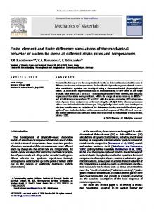
2. MODELS AND COMPUTER PROGRAMS USED For the reactor of ATUCHA I a FD model in X-Y-Z geometry was elaborated with 4 regions per channel, as shown in Fig. 1, where each hexagonal cell is covered by 4 rectangular elements. Also a lattice with 16 elements per channel was tried (twice the number of vertical and horizontal lines). For the axial direction 10 or 20 intervals were used. For the oblique control rods representation incremental cross sections are evaluated in two half cells nearest to the rod at each axial piece and at each axial level. In Fig. 1 and 2 one half and one sixth of the core is shown, but in both codes the whole reactor (symmetry 1) was calculated. The FE Lattice is performed using the fuel channels hexagonal super elements (up to a 5th degree in XY plane and 2nd degree in axial direction), complemented at the reflector zone with quadrilateral and triangular shapes, as shown in Fig. 2. The axial direction was divided into 10 pieces.
Figure 1. Rod Position for six Oblique Rods for a FD Cartesian Lattice for PUMA for the Upper Part of the Core.
Figure 2. FE lattice used for DELFIN for one Sixth of the Core.
For the FD calculation the code PUMA [3] is employed, a multigroup reactor code solving the diffusion FD equation. It is used for the fuel management at the nuclear power plants of ATUCHA I and EMBALSE. The code PUMA can also simulate power cycles (Xenon oscillations) and space kinetics using a simple double phase thermohydraulic model. For the FE calculation the code DELFIN [4] is used, a FE reactor and multicell code. It has the possibility of considering the heterogeneous properties of the cells by many ways, one of them using coefficients giving the relation between the mean fluxes at each face of them to the mean value at the whole element. So it permits to establish improved flux and current continuity among all fuel elements and especially between core and reflector zones. This improves the prediction of channel powers in peripheral channels, where a homogeneous FD code shows a slight overestimation, as we will see in the next paragraphs. DELFIN was verified with critical zero power experiments of ATUCHA I performed in 1974 and measurements in experimental critical facilities. Cell cross sections were calculated with
INAC 2005, Santos, SP, Brazil.
WIMS and supercell incremental cross sections with the Canadian code DRAGON [4]. It can also do fuel management calculations, power cycles and space kinetics with thermo hydraulic feedback. Fuel assemblies of reactors of the Nuclear Power Plants of ATUCHA I and ATUCHA II consist in 36 or 37 pin bundles in a tube of radius 5.7 cm arranged in a hexagonal lattice of a 27.2 cm pitch. Control rods are introduced into the reactor in an oblique direction as shown from above in Fig. 1 and are made of steel (gray rods) and hafnium (black rods). The ATUCHA I model has 253 fuel assemblies and ATUCHA II has 451 fuel assemblies.
Table 1. Comparison of DELFIN and PUMA with MCNP5 without Rods. Channel MCNP DELFIN PUMA Err(PUMA) Err(DLF)
K17 9.183 9.116 9.049 -1.46 -0.73
K19 L20 K21 L22 K23 M23 L24 K25 M25 8.993 8.591 8.511 8.022 7.775 7.290 7.178 6.769 6.376 8.960 8.653 8.501 8.053 7.761 7.333 7.192 6.779 6.377 8.896 8.593 8.443 8.002 7.715 7.293 7.154 6.747 6.350 -1.08 0.02 -0.80 -0.25 -0.77 0.04 -0.33 -0.33 -0.41 -0.37 0.72 -0.12 0.38 -0.18 0.59 0.19 0.15 0.02
L26 6.110 6.114 6.092 -0.29 0.07
K27 N26 M27 5.626 5.343 5.219 5.604 5.356 5.234 5.588 5.344 5.223 -0.68 0.02 0.08 -0.39 0.24 0.29
Channel MCNP DELFIN PUMA Err(PUMA) Err(%)
L28 4.873 4.874 4.868 -0.10 0.02
K29 4.320 4.294 4.297 -0.53 -0.61
K33 1.617 1.601 1.657 2.47 -1.00
O31 1.841 1.840 1.891 2.72 -0.05
N28 4.184 4.183 4.186 0.05 -0.02
M29 3.965 3.962 3.968 0.08 -0.08
L30 3.536 3.529 3.544 0.23 -0.20
K31 2.931 2.916 2.940 0.31 -0.51
O29 3.016 3.012 3.038 0.73 -0.13
Mean Quadratic Error (DELFIN) = 0.418 KEFF (MCNP) 1.00573 KEFF (DELFIN)
N30 2.925 2.915 2.941 0.55 -0.34
M31 2.641 2.626 2.655 0.53 -0.57
L32 2.189 2.182 2.225 1.64 -0.32
N32 1.677 1.669 1.721 2.62 -0.48
M33 1.358 1.356 1.408 3.68 -0.15
Mean Quadratic Error (PUMA) = 1.296 1.00470 KEFF (PUMA) 1.00511
3. CORE WITHOUT RODS Comparisons were made for an idealized core without rods (with 12.7 ppm B in the moderator, cold and 37 pins for clusters) between DELFIN, PUMA and MCNP5. Results can be seen in table 1 (channel identification shown in Fig. 1). Differences between PUMA and MCNP are small everywhere except at the periphery, where are slightly greater because of deficient treatment of flux continuity at the interface between core and reflector by the FD homogeneous model. Even so, these differences of PUMA values with the reference case are acceptable. For the case of DELFIN, the better agreement is because at each hexagonal face the relation between average cell fluxes to surface flux is used to establish continuity condition at the interface between core and reflector. 4. CORE WITHOUT SEVEN CENTRAL CHANNELS The calculation of power distribution without seven central channels (table 2) shows us a better agreement for DELFIN in channels surrounding voided central region. In this place PUMA does not treat well the interfaces, so greater differences were to be expected. This result occurs everywhere where the cell condition of periodicity is not valid.
INAC 2005, Santos, SP, Brazil.
However, DELFIN’s result is not the ideal one because there are other factors to be taken into account, such as spectral changes, and perhaps the two group theory is not very accurate. This case must be analyzed with more detail, using more energy groups or with a better spatial lattice. Normally, the reactor works with all its fuel elements, and since it is not a very frequent case, the differences obtained can be considered acceptable.
Table 2. Comparison DELFIN – PUMA - MCNP for seven empty central channels
MNCP DELFIN PUMA ERR(P) ERR(D)
K17 K19 L20 K21 L22 K23 M23 L24 K25 M25 L26 K27 0.000 0.000 6.820 6.985 7.207 7.281 7.191 7.169 7.003 6.737 6.548 6.175 0.000 0.000 7.010 7.080 7.238 7.286 7.234 7.188 6.995 6.745 6.557 6.149 0.000 0.000 7.220 7.256 7.322 7.321 7.231 7.170 6.949 6.701 6.503 6.091 0.00 0.00 5.87 3.88 1.59 0.55 0.55 0.01 –0.77 –0/53 –0.68 –1.36 0.00 0.00 2.71 1.34 0.43 0.07 0.59 0.26 -0.11 0.12 0.14 -0.42
N26 5.915 5.935 5.886 –0.49 0.34
M27 5.830 5.825 5.774 –0.96 -0.09
MNCP DELFIN PUMA ERR(P) ERR(D)
L28 5.503 5.489 5.442 –1.10 -0.26
N32 2.017 2.000 2.032 0.75 -0.85
M33 1.645 1.629 1.669 1.46 -0.98
K29 4.966 4.917 4.884 –1.66 -1.00
N28 4.801 4.803 4.751 –1.05 0.04
M29 4.588 4.574 4.536 –1.14 -0.31
L30 4.143 4.111 4.091 –1.25 -0.78
Mean Quadratic Error (DELFIN) = 0.845 KEF (DELFIN) 1.00137
K31 3.471 3.435 3.425 -1.32 -1.05
O29 3.540 3.542 3.516 -0.67 0.06
N30 3.458 3.434 3.428 –0.88 -0.70
M31 3.133 3.108 3.109 –0.77 -0.80
L32 2.617 2.598 2.614 –0.13 -0.73
K33 1.947 1.919 1.968 1.08 -1.46
O31 2.208 2.201 2.224 0.72 -0.32
Mean Quadratic Error (PUMA) = 1.61 KEF (PUMA) 1.00286
5. CORE WITH SIX OBLIQUE BLACK OR GRAY RODS Results can be seen in tables 3 and 4. As in all cases, PUMA cannot evaluate well powers at the peripheral channels. That makes its mean quadratic error greater than DELFIN´s value. However, if we observe differences for total power in channels N26 and O25 near the rods the PUMA values are a little better. That happens because the PUMA model with 20 pieces and vertical parallelepipeds simulating oblique control rods has a better precision. In other words, PUMA calculates a little better at the neighborhood of the rods while DELFIN obtains better results at the external boundary of the core. In figures 3 and 4, axial specific power distributions for channels N6 and O25 are shown for DELFIN, PUMA and MCNP for black rods. The coincidence between the three codes in both cases shows us that DELFIN and PUMA models provide a very good evaluation of the power distribution in channels near to the rods. Only in figure 4 we can see slightly greater differences between PUMA and MCNP for black rods. Hence, differences between DELFIN and MCNP are not very important. Although the greater differences appear for the black rods, as they normally are not too deep introduced, this fact is not very important. For PUMA, also a model with 4 elements per fuel channel and 10 axial pieces (not shown here) can be used, especially if it is necessary to perform a large number of flux calculations as in Xenon cycles or spatial kinetics
INAC 2005, Santos, SP, Brazil.
Table 3. Comparison DELFIN – MCNP - PUMA for six oblique black rods. Channel MCNP DELFIN PUMA Err PUMA Err DLF
K17 10.013 10.001 9.892 -1.21 0.12
K19 9.811 9.787 9.681 -1.33 -0.24
L18 9.721 9.777 9.676 -0.46 0.58
K21 9.166 9.169 9.073 -1.02 0.03
L20 9.326 9.354 9.257 -0.74 0.30
M19 9.073 9.123 9.037 -0.40 0.56
K23 8.216 8.216 8.139 -0.94 -0.00
L22 8.522 8.548 8.462 -0.70 0.31
M21 8.481 8.503 8.416 -0.77 0.26
N20 8.062 8.095 8.025 -0.46 0.41
K25 7.070 7.049 6.997 -1.03 -0.29
Channel MCNP DELFIN PUMA Err PUMA Err DLF
N22 7.299 7.307 7.222 -1.05 -0.11
O21 6.808 6.823 6.771 -0.55 0.22
K27 5.793 5.774 5.746 -0.81 -0.33
L26 6.240 6.240 6.206 -0.55 -0.00
M25 6.212 6.231 6.205 -0.11 0.30
N24 5.980 6.036 5.941 -0.66 0.94
O23 5.974 5.961 5.896 -1.31 -0.22
P22 5.482 5.478 5.446 -0.66 -0.08
K29 4.436 4.424 4.418 -0.40 -0.28
L28 4.975 4.970 4.956 -0.39 -0.10
M27 N26 O25 5.157 4.838 4.732 5.156 4.896 4.728 5.132 4.853 4.716 -0.48 0.32 -0.33 -0.03 1.19 -0.09
Channel MCNP DELFIN PUMA Err PUMA Err DLF
P24 4.666 4.640 4.623 -0.93 -0.57
Q23 4.152 4.144 4.131 -0.50 -0.20
M29 3.968 3.956 3.965 -0.08 -0.31
N28 O27 P26 Q25 R24 4.007 3.767 3.628 3.391 2.823 3.996 3.811 3.649 3.366 2.816 3.992 3.771 3.621 3.366 2.824 -0.37 0.11 -0.18 -0.73 0.02 -0.28 1.17 0.57 -0.72 -0.24
K33 1.674 1.661 1.716 2.53 -0.80
L32 2.259 2.249 2.292 1.47 -0.44
M31 2.680 2.662 2.689 0.34 -0.69
Channel MCNP DELFIN PUMA Err PUMA Err DLF
P28 2.703 2.637 2.707 0.16 -2.46
Q27 2.488 2.458 2.488 0.01 -1.21
R26 2.113 2.088 2.123 0.45 -1.17
S25 1.551 1.545 1.595 2.82 -0.38
Q29 1.590 1.568 1.622 1.99 -1.37
R28 1.305 1.289 1.339 2.63 -1.21
Mean Quadratic Error DELFIN = 0.519 Mean Quadratic Error PUMA = 0.76
M33 1.399 1.389 1.439 2.89 -0.75
N32 1.686 1.673 1.722 2.15 -0.79
KEFF DELFIN KEFF MCNP
O31 1.800 1.792 1.840 2.23 -0.44
P30 1.760 1.745 1.795 2.00 -0.85
1.00027 0.99826
KEFF PUMA
L24 7.440 7.454 7.394 -0.62 0.18
N30 2.884 2.870 2.891 0.24 -0.47
M23 7.464 7.488 7.404 -0.80 0.32
O29 2.872 2.857 2.873 0.05 -0.51
1.00097
Table 4. Comparison DELFIN - MCNP for six oblique gray rods. Channel MCNP DELFIN PUMA Err PUMA Err DLF
K17 9.762 9.746 9.626 -1.39 -0.16
K19 9.573 9.550 9.435 -1.44 -0.24
L18 9.496 9.542 9.432 -0.67 0.49
K21 8.991 8.981 8.879 -1.25 -0.11
L20 9.139 9.156 9.050 -0.97 0.18
M19 8.903 8.949 8.854 -0.55 0.52
K23 8.095 8.095 8.013 -1.01 0.01
L22 8.397 8.415 8.326 -0.85 0.21
M21 8.368 8.383 8.293 -0.90 0.17
N20 7.978 8.009 7.933 -0.56 0.39
K25 6.984 6.986 6.927 -0.82 0.03
Channel MCNP DELFIN PUMA Err PUMA Err DLF
N22 7.280 7.289 7.209 -0.97 0.13
O21 6.806 6.822 6.769 -0.55 0.24
K27 5.757 5.738 5.703 -0.93 -0.33
L26 6.212 6.221 6.178 -0.55 0.14
M25 6.276 6.297 6.264 -0.19 0.34
N24 6.110 6.156 6.078 -0.53 0.75
O23 6.019 6.018 5.961 -0.97 -0.01
P22 5.513 5.521 5.491 -0.40 0.15
K29 4.418 4.395 4.384 -0.78 -0.53
L28 4.952 4.954 4.933 -0.38 0.04
M27 N26 O25 5.189 4.997 4.874 5.194 5.036 4.872 5.167 5.004 4.863 -0.42 0.14 -0.23 0.09 0.78 -0.05
Channel MCNP DELFIN PUMA Err PUMA Err DLF
P24 4.727 4.715 4.695 -0.67 -0.26
Q23 4.181 4.185 4.178 -0.07 0.09
M29 3.979 3.972 3.969 -0.26 -0.18
N28 O27 P26 Q25 R24 4.064 3.879 3.719 3.427 2.844 4.058 3.883 3.708 3.405 2.836 4.051 3.884 3.713 3.415 2.855 -0.33 0.14 -0.16 -0.34 0.38 -0.14 0.09 -0.30 -0.65 -0.27
K33 1.660 1.648 1.699 2.35 -0.75
L32 2.246 2.235 2.272 1.15 -0.49
M31 2.672 2.658 2.678 0.24 -0.54
Channel MCNP DELFIN PUMA Err PUMA Err DLF
P28 2.760 2.739 2.767 0.25 -0.76
Q27 2.528 2.501 2.531 0.10 –1.07
R26 2.125 2.113 2.149 1.13 -0.54
S25 1.564 1.560 1.611 3.02 -0.24
Q29 1.615 1.594 1.648 2.05 -1.28
R28 1.319 1.306 1.357 2.85 -0.97
Mean Quadratic Error (DELFIN) = 0.408 Mean Quadratic Error (PUMA) = 0.78
INAC 2005, Santos, SP, Brazil.
M33 1.387 1.382 1.430 3.13 -0.39
N32 1.685 1.674 1.721 2.11 -0.67
O31 1.817 1.806 1.854 2.04 -0.59
KEFF DELFIN KEFF MCNP
P30 1.781 1.771 1.821 2.23 -0.56
1.00274 1.00047
KEFF PUMA
L24 7.374 7.394 7.328 -0.62 0.27
N30 2.905 2.882 2.906 0.02 -0.81
M23 7.439 7.459 7.382 -0.77 0.27
O29 2.920 2.886 2.919 -0.03 -1.18
1.00331
Figure 3. Channel O25. Oblique Black Rods. Axial Power Distribution
Figure 4. Channel N26. Oblique Black Rods. Axial Power Distribution
6. CONCLUSIONS - All cases show us that PUMA has difficulties to represent well interfaces between core and reflector. That is the reason why the mean quadratic error of PUMA is always a little greater than DELFIN’s. In spite of this fact, we can say that PUMA results in X-Y-Z are good. - When control rods exist, the model implemented in PUMA with parallelepipeds and 20 axial pieces provides a very good result around the rods, slightly better than DELFIN’s, which is anyway acceptable. - For empty channels some of the obtained results do not satisfy us completely. Even so, since it is not a very frequent case, they are acceptable. - Both the X-Y-Z FD model and the FE model can be considered reliable for any kind of reactor calculation: fuel element management, Xenon simulation or spatial kinetics. REFERENCES 1. F. Leszczynski, “Reference 2D and 3D Montecarlo Calculations of Idealized Cases of a Heavy Water Reactor for Benchmark Comparisons with Results from Deterministic Methods”, paper presented in this conference. 2. C. Grant, “Manual del Código PUMA Versión 4”, CNEA, C.RCN.MUS.059. 27-12-2004 3. C. Grant, “Elementos Finitos Homogéneos y Heterogéneos para la Simulación de Reactores Nucleares”, CNEA, CAYAN, I.T. 1009/92. 4. G. Marleau, A. Herbert and R.Roy. A user guide for DRAGON. Version DRAGON_000331 release 3.04. Technical report. IGE-174 Rev.5. April 2000. 5. X-5 Montecarlo Team. MCNP- A general Monte Carlo N-particle transport code, version 5. Volume II: User´s Guide. LA-CP-03-0245. 2003.03.24.
INAC 2005, Santos, SP, Brazil.