curable in communication system. For a linear ... function of the system becomes, d tj eq ...... [6] Simon Haykin, âAdaptive Filter Theoryâ, Fourth Edition, Pearson.
IACSIT International Journal of Engineering and Technology, Vol.3, No.1, February 2011 ISSN: 1793-8236
Comparison of LMS and FDAF Algorithms in Equalization of Fading Channel Md. Imdadul Islam, Md. Ariful Islam, Nur Mohammad, Mahbubul Alam, and M.R. Amin, Member, IEEE
Abstract—Wireless link in mobile cellular communication system is experienced by large and small scale fading. Since the link is Non Line of Sight (NLOS), therefore, severely affected by multipath fading. Adaptive equalizer is a widely used technique to neutralize the effect of multipath fading. In this paper, Frequency Domain Adaptive Filer (FDAF) and Least Mean Square (LMS) algorithms are used to combat the effect of multipath fading for 16-QAM and QPSK modulated wave and the results are shown using constellation diagram and bit error rate (BER). Finally, a comparison is made between two algorithms in contexts of process time, mean BER, variance of BER and circuit complexity. Index Terms—Mobile cellular communications, fading channel, channel equalization, adaptive equalizer.
I. INTRODUCTION In large scale propagation model, the separation between transmitter and receiver is very large and the link is almost line-of-sight (LOS), where only the effect of reflection, diffraction and scattering of electromagnetic (EM) wave is considered to measure the performance of a link theoretically. On the other hand, small scale fading is used to describe the rapid fluctuations of the amplitudes, phases or multi-path delays of a radio signal over a short period of time or traveled distance [1-3]. Fading is responsible for multipath propagation, speed of mobile, speed of surrounding objects and transmission bandwidth of the channel. Any passband signal is received as the sum of attenuated and delayed version of the original signal under a fading channel. Most of the cases, the impulse response of the channel is found time selective, i.e. the channel is better at selected times than other times [4,5]. To neutralize the delay spread of wireless channel, adaptive equalizer is used on passband signal [1,5]. In this paper, two well known adaptive algorithms: least mean square (LMS) algorithm and frequency domain adaptive filter (FDAF) algorithm are used in equalizer circuit at the receiving end of the wireless link. These algorithms are widely used in adaptive noise cancellation but adaptive equalization is a real time signal processing system, therefore, choice of optimum algorithm taking BER as a constraint is a Manuscript received October 23, 2010. Md. Imdadul Islam, Md. Ariful Islam, Nur Mohammad, and Mahbubul Alam are with the Computer Sciencen and Engineering Department, Jahangirnagar University, Savar, Dhaka 1342, Bangladesh. M. R. Amin is with the Department of Electronics and Communications Engineering, East West University, 43 Mohakhali, Dhaka 1212, Bangladesh (corresponding author, phone: +880-1715296735; fax: +880-2-8812336; e-mail: ramin@ ewubd.edu).
16
complicated task. The choice of algorithm may change with changing modulation scheme and the amount of fading introduced by the channel. In this paper, 16-QAM and QPSK modulation schemes are used to find scattered diagram and BER for the cases of with and without equalization. Here, the above mentioned two algorithms are compared considering process time of the algorithms, mean error, variance of error, and complexity of circuit implementation. Both algorithms are simpler compared to other adaptive algorithms, for example, Recursive Least Square (RLS) and Kalman Filter [6,7]. The paper is organized as follows. Section II gives the theoretical analysis of the adaptive equalizer and adaptive algorithm (LMS and FDAF), section III gives the results where constellation diagram of received symbols (16-QAM and QPSK) for the cases of with and without equalization, BER and a comparison of two algorithms are made. Finally section IV concludes the paper. II. THEORETICAL ANALYSIS A. Adaptive Equalizer If any signal x(t ) is multiplied by a constant k or delayed by an amount t d , then the resultant signal becomes
k x(t − t d ) . Such distortion is called linear distortion and is
curable in communication system. For a linear distortion channel of Fig.1, the equalizer output can be written as y (t ) = k x(t − t d ) . Taking Fourier transform, we have Y ( f ) / X ( f ) = ke − jωtd = H ( f ) . In presence of distorting
channel of transfer function H c ( f ) , the received signal can be made distortionless by incorporating an equalizer at the receiving end as shown in Fig. 1. The overall transfer function of the system becomes, H c ( f ) H eq ( f ) = ke − jωtd , where H ( f ) is called the amplitude response function and need to be a constant over the entire bandwidth (BW) of the input signal, and θ ( f ) is the phase response need to be a linear function of frequency over the entire BW of the input signal for recovery transmitted symbol [8-10]. Let us consider the tapped delay FIR filter of Fig. 2, where the output signal is y (t ) = C − N x(t ) + C − N +1 x(t − τ ) + C − N + 2 x(t − 2τ ) + L + C 0 x(t − Nτ ) + L + C N x(t − 2 Nτ ).
IACSIT International Journal of Engineering and Technology, Vol.3, No.1, February 2011 ISSN: 1793-8236 Communication Channel, Hc(f)
Equalizer, Heq(f)
x(t)
y(t)
Fig. 1 Equalizer in cascade with the channel.
x(t)
τ
×
C-N
x(t- τ)
C-N+1
×
x(t- 2τ)
τ C-N+2
×
…… ……
…… ……
τ
C0
x(t2Nτ)
CN
×
…… ……
τ
×
…… ……
Σ y(t) Fig. 2 Tapped delay line equalizer.
Let us consider the tapped delay FIR filter of Fig. 2, where the output signal is y (t ) = C − N x(t ) + C − N +1 x(t − τ ) + C − N + 2 x(t − 2τ ) + L + C 0 x(t − Nτ ) + L + C N x(t − 2 Nτ ).
adjusting the number of delay blocks and weighting factors of Eq. (1), then distortion at receiving end can be eliminated [11]. Example A simple multipath (here for simplicity, we consider only two paths) propagation scenario is shown in Fig. 3. Let us determine the weighting factors of 3 tapped delay equalizer for distortion less received signal. Here, the received signal is y (t ) = k1 x(t − t1 ) + k 2 x(t − t 2 ) . Thus, after Fourier transformation, Y ( f ) = k1 X ( f )e − jωt1 + k2 X ( f )e− jωt2 , which gives
Taking Fourier transform, we have Y ( f ) = C − N X ( f ) + C − N +1 X ( f )e − jωτ + C − N + 2 X ( f )e − j 2ωτ + ... ... ... + C 0 X ( f )e − jNωτ + ... ... ... + C N X ( f )e − j 2 Nωτ , and from which, we have
(
Reflector
where k = k 2 / k1 and t 0 = t 2 − t1 . We require, H eq ( f ) H c ( f ) = k1e − jωt1 , from which we can write
k2x(t-t2)
k1x(t-t1)
H eq ( f ) =
Radio tow er
= =
After expanding,
Fig. 3 Two path wave propagation.
H eq ( f ) =
Y( f ) = e − jNωτ X(f )
If relation H c ( f ) H eq ( f ) = ke
n=− N − jω t d
k1e− jωt1 Hc ( f ) k1e− jωt1
(
k1e− jωt1 1 + ke− jωt0 1
(1 + ke
− jωt0
)
).
H eq ( f ) = 1 − ke − jωt0 + k 2 e − j 2ωt0 − ... ... ...
N
∑ C n e − j 2π f nτ .
)
Y( f ) = H c ( f ) = k1e − jω t1 + k 2 e − jω t2 = k1e − jωt1 1 + ke − jωt0 , X(f )
(1)
can be satisfied by 17
or H eq ( f ) ≈ 1 − ke − jωt0 + k 2 e − j 2ωt0 .
Therefore, C −1 = 1 , C 0 = −k and C1 = k 2 .
IACSIT International Journal of Engineering and Technology, Vol.3, No.1, February 2011 ISSN: 1793-8236
B. Frequency Domain Adaptive Filter (FDAF) technique Let L is the length of the block and M is the length of tapped weight vector. Let ⎡ u (kL) ⎤ ⎡ u (kL − 1) ⎤ ⎢ u (kL + 1) ⎥ ⎢ ⎥ ⎥ , A = ⎢ u (kL) ⎥ , …, A0 = ⎢ 1 ⎢ ⎢ ⎥ ⎥ L L ⎢ ⎢ ⎥ ⎥ ⎣u (kL + L − 1)⎦ ⎣u (kL + L − 2)⎦ ⎡ u (kL − 1) ⎤ ⎥ ⎢ u (kL) ⎥. A M −1 = ⎢ ⎥ ⎢ L ⎥ ⎢ ⎣u (kL + L − 2)⎦ The data matrix can then be written as A(k ) = [A 0 A1 A 2 L A M −1 ] ⎡G (kM ) ⎢G (kM + 1) =⎢ ⎢... ⎢ ⎣G (kM + L − 1 The matrix A(k ) is an L × M
⎤ ⎥ ⎥. (2) ⎥ ⎥ ⎦ matrix and length of the
vector G T (kM ) is M. Let the weight vector be ˆ (k ) = [ w (k ) W 0
w1 (k )
w2 (k ) ... w L −1 (k )]T .
(3)
Output of the filter is y (kL + 2) ... y (kL + L − 1)]T
y (kL + 1) ˆ (k ) = A(k ).W
[ y (kL)
.
(4)
For individual element, y (kL) = G (kM ).Wˆ (k ) y (kL + 1) = G (kM + 1).Wˆ (k )
w1 (k )
j
[ y (kL + L) y (kL + L + 1) y (kL + L + 2) ... y (kL + 2 L − 1)]T (9) ˆ (k + 1). = A(k + 1).W
The updated error matrix ⎤ ⎡ y (kL + L) ⎤ ⎡e(kL + L) ⎡d (kL + L) ⎢d (kL + L + 1) ⎥ ⎢ y (kL + L + 1) ⎥ ⎢e(kL + L + 1) ⎥ ⎢ ⎥ ⎢ ⎢ ⎢d (kL + L + 2) ⎥ ⎢ y (kL + L + 2) ⎥ ⎢e(kL + L + 2) ⎥ ⎢ ⎥ ⎢ ⎢ ⎥ - ⎢ ... ⎥ = ⎢ ... ⎢ ... ⎥ ⎢... ⎥ ⎢... ⎢... ⎥ ⎢ ⎥ ⎢ ⎢ ⎥ ⎢... ⎥ ⎢... ⎢... ⎢d (kL + 2 L − 1) ⎥ ⎢ y (kL + 2 L − 1) ⎥ ⎢e(kL + 2 L − 1) ⎦ ⎣ ⎦ ⎣ ⎣
is ⎤ ⎥ ⎥ ⎥ ⎥ ⎥ ⎥ ⎥ ⎥ ⎥ ⎦
(11)
and ˆ ( k + 2) = W ˆ (k + 1) + μΦ(k + 1) . W
(12)
Similarly, [ y (kL + iL ) y (kL + iL + 1) y (kL + iL + 2) ... ˆ (k + i) . y (kL + (i + 1) L − 1)]T = A(k + i ).W
M −1 j =0
(7) The update equation of the weight vector can be written as ˆ (k + 1) = W ˆ (k ) + μΦ(k ) , W (8) where μ is the step-size parameter. ˆ (k + 1) , we have Now using W
Φ(k + 1) = A T (k + 1)e(k + 1) ,
w2 (k ) ... ... ... w L −1 (k )]
∑ w (k ).u (kL + i − j ) .
Φ(k ) = A T (k )e(k ) .
(10) The updated cross correlation vector and the weight vector are respectively as
u (kL + i) ⎡ ⎤ ⎢ u (kL + i − 1) ⎥ ⎢ ⎥ × ⎢ u (kL + i − 2) ⎥ ⎢ ⎥ M ⎢ ⎥ ⎢⎣u (kL + i + M − 1)⎥⎦
=
(6) The cross correlation vector is
= e(k + 1) .
……………………………. y (kL + i ) = G (kM + i ).Wˆ (k ) = [ w0 ( k )
⎡d (kL) ⎤ ⎡ y (kL) ⎤ ⎡e(kL) ⎤ ⎢d (kL + 1) ⎥ ⎢ y (kL + 1) ⎥ ⎢e(kL + 1) ⎥ ⎢ ⎥ ⎢ ⎥ ⎢ ⎥ ⎢d (kL + 2) ⎥ ⎢ y (kL + 2) ⎥ ⎢e(kL + 2) ⎥ ⎢ ⎥ ⎢ ⎥ ⎢ ⎥ ⎢ ... ⎥ - ⎢ ... ⎥ = ⎢ ... ⎥ = e(k ) . ⎢... ⎥ ⎢... ⎥ ⎢... ⎥ ⎢ ⎥ ⎢ ⎥ ⎢ ⎥ ⎢... ⎥ ⎢... ⎥ ⎢... ⎥ ⎢d (kL + L − 1)⎥ ⎢ y (kL + L − 1)⎥ ⎢e(kL + L − 1)⎥ ⎣ ⎦ ⎣ ⎦ ⎣ ⎦
(5)
Let the desired response of (kL + i ) − th element is
d (kL + i ) . Therefore, the error signal is e(kL + i ) = d (kL + i ) − y (kL + i ) . In matrix form,
18
Let ⎤ ⎤ ⎡ y (kL + iL ) ⎡d (kL + iL) ⎥ ⎥ ⎢ y (kL + iL + 1) ⎢d (kL + iL + 1) ⎥ ⎥ ⎢ ⎢ ⎥ ⎥ ⎢ y (kL + iL + 2) ⎢d (kL + iL + 2) ⎥ ⎥ ⎢ ⎢ ⎥ ⎥ − ⎢ ... ⎢ ... ⎥ ⎥ ⎢... ⎢... ⎥ ⎥ ⎢ ⎢ ⎥ ⎥ ⎢... ⎢... ⎢d (kL + (i + 1) L − 1)⎥ ⎢ y (kL + (i + 1) L − 1)⎥ ⎦ ⎦ ⎣ ⎣
(13)
IACSIT International Journal of Engineering and Technology, Vol.3, No.1, February 2011 ISSN: 1793-8236
⎤ ⎡e(kL + iL) ⎥ ⎢e(kL + iL + 1) ⎥ ⎢ ⎥ ⎢e(kL + iL + 2) ⎥ ⎢ = ⎢ ... ⎥ = e( k + i ) . ⎥ ⎢... ⎥ ⎢ ⎥ ⎢... ⎢e(kL + (i + 1) L − 1)⎥ ⎦ ⎣
ˆ (k + 1) = W ˆ (k ) + μFFT ⎡φ(k )⎤ . W ⎢O ⎥ ⎦ ⎣ (14)
In generalized form, Φ(k + i ) = A T (k + i )e(k + i ) ,
(15)
and ˆ (k + i + 1) = W ˆ (k + i) + μΦ(k + i ) . W
(16) In overlap-save method N=2M point FFT is used and the size of the filter of M tap weights. Input signal in n domain is express as, [(k − 1)th block, kth block] , where the (k-1)-th block is ⎡u(kL− L) u(kL− L −1) u(kL− L − 2) ... ... ... u(kL− 2M +1) ⎤ ⎢u(kL− L +1) u(kL− L) u(kL− L −1) ... ... ... u(kL− L − 2M + 2)⎥⎥ ⎢ , ⎥ ⎢... ... ... ... ... ... ... ⎥ ⎢ u(kL− 2) u(kL−3) ... ... ... u(kL− 2M) ⎦ ⎣u(kL−1)
(23)
C. LMS Algorithm Least mean square filter is a type of digital adaptive filter where a desired filter is obtained by finding the filter coefficients that relate to producing the least mean squares of the error signal. In LMS, error estimation is determined by comparing the output of the linear filter in response to the input signal to the desired response. LMS then involves an adaptive process for automatic adjustment of the parameters of the filter according to the error estimation. The filtering process of LMS algorithm is performed by a transversal filter and the adaptive process is carried out by a weight control mechanism [1-4]. LMS algorithm can be summarized as follows based upon wide-sense stationary stochastic signal [8,13,14]. Parameters: M = number of tapes, µ = step-size parameter; where 0 < µ < 2 / MS max , Smax is the maximum value of
the power spectral density of the tap input u(n) and filter length M is moderate to large. Initialization: ˆ ( n) If prior knowledge of the tap-weight vector w
aAnd the k-th block is
is
ˆ ( 0) ; available, it is used to select an appropriate value of w u(kL−1) u(kL− 2) ⎡u(kL) ⎢u(kL+1) u(kL) u(kL−1) ⎢ ⎢... ... ... ⎢ u ( kL + M − 1 ) u ( kL + M − 2 ) u (kL+ M − 3) ⎣
... ... ... u(kL− 2M +1)⎤ ... ... ... u(kL− 2M + 2)⎥⎥ . ⎥ ... ... ... ... ⎥ ... ... ... u(kL− M ) ⎦
Input signal in k domain, U(k ) = diag (FFT [(k − 1)th block, kth block ])
;
ˆ (0) = 0 is set. otherwise w
an
N × N matrix. The initial weight in k domain is a N × 1 vector: ˆ ˆ (k ) = FFT ⎡w (k )⎤ . (17) W ⎢ ⎥ ⎣O ⎦ ˆ (k ) is tap-weight vector (in n domain) of length M Here w
and O is a null vector of length M. Output signal of the filter in k domain is ˆ (k )] . (18) yˆ (k ) = Last M elements of IFFT [U(k ) W The desired response vector, d(k ) = [d (kM ), d (kM + 1), ... d (kM + M − 1]T .
(19)
Error signal vector in n domain,
e(k ) = [e(kM ), e(kM + 1), ... ... ..., e(kM + M − 1]T = d(k ) − y (k ). The error signal in the frequency domain is ⎡O ⎤ E(k ) = FFT ⎢ ⎥. ⎣e(k )⎦
The cross-correlation vector is
[
(20)
(21)
]
φ(k ) = First M elements of IFFT U H (k )E(k ) . (22) Thus, the updated tap-weights [6,7,12] can be written as
19
Data: Given u(n) = M − by − 1 tap-input vector at time n = [u((n),u(n-1),…..,u(n-M+1))]T, d(n) = desired response at time t = n. To be computed: ˆ (n + 1) = estimate of tap-weight vector at time n+1. w Computation:
e( n) = d(n) − wˆ H (n + 1) u(n) ,
(24)
ˆ ( n + 1) = w ˆ ( n) + μ u ( n )e * ( n) . w
(25)
III. RESULTS AND DISCUSSIONS A simulation work is done generating 8192 symbols in a random manner. The constellation diagram is made for the symbols considering a multipath fading cannel of transfer function, H(z) = (z-0.4950 + j0.4950)(z- 0.7071 -j0.7071)/(z-1)(z+0.7). The constellation of 16-QAM and QPSK is shown in Fig. 4 (a)-(d) for the case of with and without equalization. The immense improvement in detection of symbols is visualized from the Fig. 4. Next, the simulation work is done to determine BER of both modulation schemes for the case of FDAF and LMS algorithms. In this case, 8192 symbols are generated in a random manner and BER is evaluated varying SNR form 0dB to 5dB. The simulation program is run 10 times and average BER is taken for each point of graphs of Fig. 5. In FDAF, BER has rapid fluctuation but for the case of LMS, BER is almost constant. The time taken for convergence is smaller in LMS compared to FDAF but once attaining convergence, the FDAF provides better
IACSIT International Journal of Engineering and Technology, Vol.3, No.1, February 2011 ISSN: 1793-8236
performance as it is visualized from Fig. 5. The performance of QPSK is better than that of 16-QAM for both the algorithms and the phenomenon can be explained from signal space concept.
Equalized signal y[n] 5 4 3 2
Received signal x[n] 40
Im{y[n]}
1 30 20
-1 -2
10 Im{x[n]}
0
-3
0
-4 -10
-5 -5
-20
-30
-20
-10
0 10 Re{x[n]}
20
30
5
(d) QPSK after equalization Fig. 4 Constellations of 16-QAM and QPSK before and after equalization.
-30 -40 -40
0 Re{y[n]}
40
BER of Adaptive Equalized Signal and Received Signal
0
10
a) 16-QAM before equalization
BER of equalized 16QAM BER of received 16QAM BER of equalized QPSK BER of received QPSK
Equalized signal y[n] 5
-1
10
BER
4 3 2
-2
10
Im{y[n]}
1 0 -1
-3
10
-2
0
5
10
15
-3
20
25 30 SNR (dB)
35
40
45
50
(a) FDAF
-4
BER of Adaptive Equalized Signal and Received Signal
-1
10
-5 -5
0 Re{y[n]}
5
(b) 16-QAM after equalization Received signal x[n] BER
20
-2
10
15 BER of equalized 16QAM BER of received 16QAM BER of equalized QPSK BER of received QPSK
10
Im{x[n]}
5 -3
10
0
0
5
10
-5
20
25 30 SNR (dB)
35
40
45
50
(b) LMS Fig.5 BER of received symbols.
-10 -15 -20 -20
15
TABLE I COMPARISON OF TWO ALGORITHMS -15
-10
-5
0 Re{x[n]}
5
10
15
20
Algorithm
(c) QPSK before equalization
LMS FDAF
Process Time (s) 30.0156 15.4219
Mean Error
Variance
Circuit Complexity
0.0688 0.0652
1.4295e-007 6.8392e-006
Simple Complex
Finally, a comparison is made between two algorithms taking total 8192 symbols of 16-QAM. The parameters are selected for the comparison as: process time, mean BER, variance of BER and circuit complexity (Table I). LMS is better in context of quicker convergence visualized from the variance of Table I and also from the graph of Fig. 5(b). The 20
IACSIT International Journal of Engineering and Technology, Vol.3, No.1, February 2011 ISSN: 1793-8236
circuit implementation of LMS algorithm is much easier compared to FDAF and can be understood from the theoretical analysis of Section II. On the other hand, FDAF is better in context of process time of operation and mean BER. In high speed data communication under fading wireless channel, we need an algorithm to process fading symbols before arrival of next symbols, hence FDAF algorithm is the best fit for such case. IV. CONCLUSION In this paper, two adaptive algorithms LMS and FDAF are compared in adaptive equalization of QPSK and 16-QAM signal under multipath fading. The results and discussions section of the paper shows the simulated result but in real life case the result will vary with location (where the experiment take place) and time because of small scale fading. The work can be extended incorporating other modulation schemes like MSK, GMSK, M-PSK etc. at the same time other adaptive algorithm like RLS and Kalman filter theory can also be examined for comparison. REFERENCES [1] [2] [3] [4] [5] [6] [7]
[8] [9] [10] [11]
[12] [13]
[14]
Theodore S. Rappaport , “Wireless Communications”, Second Edition, PHI Learning Private Ltd., New Delhi, ISBN-978-81-203-2381-0, 2002. X. Tang, M. S. Alounini and A. Goldsmith, “ Effect of channel estimation error on M-QAM BER performance in Rayleigh fading”, IEEE Trans. Commun., vol. 47, no. 12, 1999, pp. 1856-64. J. E. Padgett, C. G. Gunther, and T. Hattori, “Overview of Wireless personal communications,” IEEE Commun. Mag., vol.33, 1995, pp. 28-41. Zhiwei Zebg, “Digital Communication via Multipath fading Channel,” Cpre537x Final Project, 2000, pp. 17-22. Simon Haykin and Michael Moher, “Modern Wireless Communications”, Low Price Edition, PEARSON Education, New Delhi, ISBN 81-317-1133-1, 2007. Simon Haykin, “Adaptive Filter Theory”, Fourth Edition, Pearson Education, ISBN 81-7808-565-8, pp.-231-237, pp.-345-48, pp. 466-485. Md. Anamul Haque, AKM Kamrul Islam and Imdadul Islam, “Evaluation of Performnabce of Digital Adaptive Filters in Acoustic Echo Cancellation,” Proceedings of 12th ICCIT, Dec. 2009, pp. 215-219. K. Banovic, A. R. Esam and M. A. S. Khalid,, “A Novel RadiusAdjusted Approach for Blind Adaptive Equalization”, IEEE Signal Processing Letters, vol. 13, no. 1, 2006, pp. 37- 40. R. A. Valenzuela, “Performance of Adaptive Equalization for Indoor Radio Communications”, IEEE Trans. Commun., vol. 31, no. 3, 1989, pp. 291-293. C. R. Johnson Jr., “Admissibility in blind adaptive channel equalization,” IEEE Control System Mag., vol. 1, 1991, pp. 3-15. S. U. H. Qureshi, “Adaptive Equalization”, IEEE Procs., vol. 73, no. 9, 1985, pp. 1349-1387. Md. Anamul Haque, AKM Kamrul Islam, “Acoustic Echo Cancellation Using Digital Adaptive Filter,” Dept. of CSE, J.U., Jan. 2009. E. R. Ferrara, Jr., ‘Fast Implementation of LMS adaptive filter,’ IEE Trans. Acoust. Speech Signal Processing, vol. ASSP-28, 1980, pp. 474-475. O. P. Sharma, V. Janyani and S. Sancheti, “Recursive Least Squares Adaptive Filter a better ISI Compensator,” International Journal of Electronics, Circuits and Systems, vol. 3, no. 1, 2009, pp. 40-45.
21
Md. Imdadul Islam has completed his B.Sc. and M.Sc Engineering in Electrical and Electronic Engineering from Bangladesh University of Engineering and Technology, Dhaka, Bangladesh in 1993 and 1998 respectively and has completed his Ph.D degree from the Department of Computer Science and Engineering, Jahangirnagar University, Dhaka, Bangladesh in the field of network traffic engineering. He is now working as a Professor at the Department of Computer Science and Engineering, Jahangirnagar University, Savar, Dhaka, Bangladesh. Previously, he worked as an Assistant Engineer in Sheba Telecom (Pvt.) LTD (A joint venture company between Bangladesh and Malaysia, for Mobile cellular and WLL), from Sept'94 to July'96. He has a very good field experience in installation of Radio Base Stations and Switching Centers for WLL. His research field is network traffic, wireless communications, wavelet transform, OFDMA, WCDMA, adaptive filter theory, ANFIS and array antenna systems. He has more than hundred research papers in national and international journals and conference proceedings.
Md. Ariful Islam has completed B.Sc Engineering from the Department of Computer Science and Engineering, Jahangirnagar University, Dhaka, Bangladesh in 2010.
Nur Mohammad has completed B.Sc Engineering from the Department of Computer Science and Engineering, Jahangirnagar University, Dhaka, Bangladesh in 2010. Now he is working as a programmer in Epsilonn Technologies Limited, Bangladesh. Mahbubul Alam completed his B.Sc. (Hons.) in Computer Science and Engineering from Jahangirnagar University, Savar, Dhaka, Bangladesh in 2006. He received the “Asadul Kabir Gold Medal” for securing the highest grade in the B.Sc. (Hons.) final examination 2006 at Jahangirnagar University. He is now working as a Lecturer, at the department of Computer Science and Engineering, Jahangirnagar University, Savar, Dhaka, Bangladesh from 13th July 2009. His research interests are wavelet transform, wireless communications, adaptive filter theory, artificial intelligence, image processing and machine learning. M. R. Amin received his B.S. and M.S. degrees in Physics from Jahangirnagar University, Dhaka, Bangladesh in 1984 and 1986 respectively and his Ph.D. degree in Plasma Physics from the University of St. Andrews, U. K. in 1990. He is a Professor of Electronics and Communications Engineering at East West University, Dhaka, Bangladesh. He served as a Post-Doctoral Research Associate in Electrical Engineering at the University of Alberta, Canada, during 1991-1993. He was an Alexander von Humboldt Research Fellow at the Max-Planck Institute for Extraterrestrial Physics at Garching/Munich, Germany during 1997-1999. Dr. Amin awarded the Commonwealth Postdoctoral Fellowship in 1997. Besides these, he has also received several awards for his research, including the Bangladesh Academy of Science Young Scientist Award for the year 1996 and the University Grants Commission Young Scientist Award for 1996. He is a member of the IEEE.